Artificial
Intelligence 3E
foundations of computational agents
9.6 Sequential Probability Models
Special types of belief networks with repeated structure are used for reasoning about time and other sequences, such as sequences of words in a sentence. Such probabilistic models may have an unbounded number of random variables. Reasoning with time is essential for agents in the world. Reasoning about text with unbounded size is important for understanding language.
9.6.1 Markov Chains
A Markov chain is a belief network with random variables in a sequence, where each variable only directly depends on its predecessor in the sequence. Markov chains are used to represent sequences of values, such as the sequence of states in a dynamic system or language model. Each point in the sequence is called a stage.
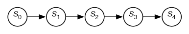
Figure 9.14 shows a generic Markov chain as a belief network. The network has five stages, but does not have to stop at stage ; it can extend indefinitely. The belief network conveys the independence assumption
which is called the Markov assumption.
Often the sequences are in time, and represents the state at time . The state conveys all of the information about the history that could affect the future. The independence assumption of the Markov chain can be seen as “the future is conditionally independent of the past given the state.”
A Markov chain is a stationary model or time-homogenous model if the variables all have the same domain, and the transition probabilities are the same for each stage:
To specify a stationary Markov chain, two conditional probabilities are provided:
-
•
specifies the initial conditions
-
•
specifies the dynamics, which is the same for each .
The sharing of the parameters for the conditional probability is known as parameter sharing or weight tying, as used in convolutional neural networks.
Stationary Markov chains are of interest for the following reasons:
-
•
They provide a simple model that is easy to specify.
-
•
The assumption of stationarity is often the natural model, because the dynamics of the world typically does not change in time. If the dynamics does change in time, it is usually because of some other feature that could also be modeled as part of the state.
-
•
The network extends indefinitely. Specifying a small number of parameters gives an infinite network. You can ask queries or make observations about any arbitrary points in the future or the past.
To determine the probability distribution of state , variable elimination can be used to sum out the preceding variables. The variables after are irrelevant to the probability of and need not be considered. To compute , where , only the variables between and need to be considered, and if , only the variables less than need to be considered.
A stationary distribution of a Markov chain is a distribution of the states such that if it holds at one time, it holds at the next time. Thus, is a stationary distribution if for each state , . Thus
Every Markov chain with a finite number of states has at least one stationary distribution. The distribution over states encountered in one infinite run (or the limit as the number of steps approaches infinity) is a stationary distribution. Intuitively, if an agent is lost at time , and doesn’t observe anything, it is still lost at time . Different runs might result in different parts of the state space being reached, and so result in different stationary distributions. There are some general conditions that result in unique stationary distributions, which are presented below.
A Markov chain is ergodic if, for any two states and , there is a nonzero probability of eventually reaching from .
A Markov chain is periodic with period if the difference between the times when it visits the same state is always divisible by . For example, consider a Markov chain where the step is per day, so is the state on the day after , and where the day of the week is part of the state. A state where the day is Monday is followed by a state where the day is Tuesday, etc. The period will be (a multiple of) 7; a state where the day is Monday can only be a multiple of 7 days from a state where the day is also Monday. If the only period of a Markov chain is a period of 1, then the Markov chain is aperiodic.
If a Markov chain is ergodic and aperiodic, then there is a unique stationary distribution, and this is the equilibrium distribution that will be approached from any starting state. Thus, for any distribution over , the distribution over will get closer and closer to the equilibrium distribution, as gets larger.
The box gives an application of Markov chains that formed the basis of Google’s initial search engine.
PageRank
Google’s initial search engine [Brin and Page, 1998] was based on PageRank [Page et al., 1999], a probability measure over web pages where the most influential web pages have the highest probability. It is based on a Markov chain of a web surfer who starts on a random page, and with some probability picks one of the pages at random that is linked from the current page, and otherwise (if the current page has no outgoing links or with probability ) picks a page at random. The Markov chain is defined as follows:
-
•
The domain of is the set of all web pages.
-
•
is the uniform distribution of web pages: for each web page , where is the number of web pages.
-
•
The transition is defined as follows:
where there are web pages and links on page . The way to think about this is that is the current web page, and is the next web page. If has no outgoing links, then is a page at random, which is the effect of the middle case. If has outgoing links, with probability the surfer picks a random page linked from , and otherwise picks a page at random.
-
•
is the probability someone picks a link on the current page.
This Markov chain converges to a stationary distribution over web pages. Page et al. [1999] reported the search engine had converged to “a reasonable tolerance” for with 322 million links.
PageRank provides a measure of influence. To get a high PageRank, a web page should be linked from other pages with a high PageRank. It is difficult, yet not impossible, to manipulate PageRank for selfish reasons. One could try to artificially boost PageRank for a specific page, by creating many pages that point to that page, but it is difficult for those referring pages to also have a high PageRank.
In the initial reported version, Brin and Page [1998] used 24 million web pages and 76 million links. The web is more complex now, with many pages being dynamically generated, and search engines use much more sophisticated algorithms.
9.6.2 Hidden Markov Models
A hidden Markov model (HMM) is an augmentation of a Markov chain to include observations. A hidden Markov model includes the state transition of the Markov chain, and adds to it observations at each time that depend on the state at the time. These observations can be partial in that different states map to the same observation and noisy in that the same state can map to different observations at different times.
The assumptions behind an HMM are:
-
•
The state at time only directly depends on the state at time for , as in the Markov chain.
-
•
The observation at time only directly depends on the state at time .
The observations are modeled using the variable for each time whose domain is the set of possible observations. The belief-network representation of an HMM is depicted in Figure 9.15. Although the belief network is shown for five stages, it extends indefinitely.
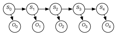
A stationary HMM includes the following probability distributions:
-
•
specifies initial conditions
-
•
specifies the dynamics or the belief state transition function
-
•
specifies the sensor model.
Example 9.30.
Suppose you want to keep track of an animal in a triangular enclosure using sound. You have three microphones that provide unreliable (noisy) binary information at each time step. The animal is either near one of the three vertices of the triangle or close to the middle of the triangle. The state has domain , where means the animal is in the middle and means the animal is in corner .
The dynamics of the world is a model of how the state at one time depends on the previous time. If the animal is in a corner, it stays in the same corner with probability 0.8, goes to the middle with probability 0.1, or goes to one of the other corners with probability 0.05 each. If it is in the middle, it stays in the middle with probability 0.7, otherwise it moves to one of the corners, each with probability 0.1.
The sensor model specifies the probability of detection by each microphone given the state. If the animal is in a corner, it will be detected by the microphone at that corner with probability 0.6, and will be independently detected by each of the other microphones with probability 0.1. If the animal is in the middle, it will be detected by each microphone with probability 0.4.
Initially the animal is in one of the four states, with equal probability.
There are a number of tasks that are common for HMMs.
The problem of filtering or belief-state monitoring is to determine the current state based on the current and previous observations, namely to determine
All state and observation variables after are irrelevant because they are not observed and can be ignored when this conditional distribution is computed.
Example 9.31.
Consider filtering for Example 9.30.
The following table gives the observations for each time, and the resulting state distribution.
| Observation | Posterior State Distribution | ||||||
| Time | Mic#1 | Mic#2 | Mic#3 | ||||
| initially | – | – | – | 0.25 | 0.25 | 0.25 | 0.25 |
| 0 | 0 | 1 | 1 | 0.46 | 0.019 | 0.26 | 0.26 |
| 1 | 1 | 0 | 1 | 0.64 | 0.084 | 0.019 | 0.26 |
Thus, even with only two time steps of noisy observations from initial ignorance, it is very sure that the animal is not at corner 1 or corner 2. It is most likely that the animal is in the middle.
Note that the posterior distribution at any time only depended on the observations up to that time. Filtering does not take into account future observations that provide more information about the initial state.
The problem of smoothing is to determine a state based on past and future observations. Suppose an agent has observed up to time and wants to determine the state at time for ; the smoothing problem is to determine
All of the variables and for can be ignored.
Localization
Suppose a robot wants to determine its location based on its history of actions and its sensor readings. This is the problem of localization.
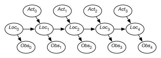
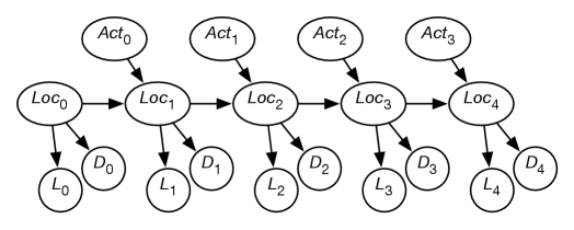
Figure 9.16 shows a belief-network representation of the localization problem. There is a variable for each time , which represents the robot’s location at time . There is a variable for each time , which represents the robot’s observation made at time . For each time , there is a variable that represents the robot’s action at time . In this section, assume that the robot’s actions are observed. (The case in which the robot chooses its actions is discussed in Chapter 12.)
This model assumes the following dynamics: at time , the robot is at location , it observes , then it acts, it observes its action , and time progresses to time , where it is at location . Its observation at time only depends on the state at time . The robot’s location at time depends on its location at time and its action at time . Its location at time is conditionally independent of previous locations, previous observations, and previous actions, given its location at time and its action at time .
The localization problem is to determine the robot’s location as a function of its observation history:
Example 9.32.
Consider the domain depicted in Figure 9.17.
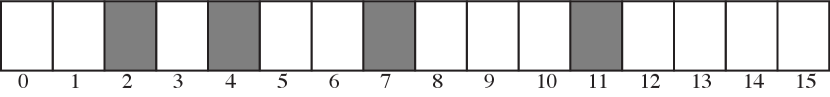
There is a circular corridor, with 16 locations numbered 0 to 15. The robot is at one of these locations at each time. This is modeled with, for every time , a variable with domain .
-
•
There are doors at positions 2, 4, 7, and 11 and no doors at other locations.
-
•
The robot has a sensor that noisily senses whether or not it is in front of a door. This is modeled with a variable for each time , with domain . Assume the following conditional probabilities:
where is true when the robot is at states 2, 4, 7, or 11 at time .
Thus, the observation is partial in that many states give the same observation and it is noisy in the following way: in 20% of the cases in which the robot is at a door, the sensor gives a negative reading (a false negative). In 10% of the cases where the robot is not at a door, the sensor records that there is a door (a false positive).
-
•
The robot can, at each time, move left, move right, or stay still. Assume that the stay still action is deterministic, but the dynamics of the moving actions are stochastic. Just because the robot carries out the action does not mean that it actually goes one step to the right – it is possible that it stays still, goes two steps right, or even ends up at some arbitrary location (e.g., if someone picks up the robot and moves it). Assume the following dynamics, for each location :
All location arithmetic is modulo 16. The action works the same way but to the left.
The robot starts at an unknown location and must determine its location.
It may seem as though the domain is too ambiguous, the sensors are too noisy, and the dynamics is too stochastic to do anything. However, it is possible to compute the probability of the robot’s current location given its history of actions and observations.
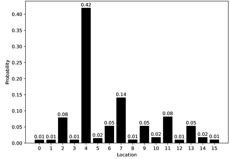
Figure 9.18 gives the robot’s probability distribution over its locations, assuming it starts with no knowledge of where it is and experiences the following observations: observe door, go right, observe no door, go right, and then observe door. Location 4 is the most likely current location, with posterior probability of 0.42. That is, in terms of the network of Figure 9.16:
Location 7 is the second most likely current location, with posterior probability of 0.141. Locations 0, 1, 3, 8, 12, and 15 are the least likely current locations, with posterior probability 0.011.
You can see how well this works for other sequences of observations using the AIPython (aipython.org) code.
Example 9.33.
Let us augment Example 9.32 with another sensor. Suppose that, in addition to a door sensor, there is also a light sensor. The light sensor and the door sensor are conditionally independent given the state. Suppose the light sensor is not very informative; it only gives yes-or-no information about whether it detects any light, and this is very noisy, and depends on the location.
This is modeled in Figure 9.19 using the following variables:
-
•
is the robot’s location at time
-
•
is the robot’s action at time
-
•
is the door sensor value at time
-
•
is the light sensor value at time .
Conditioning on both and lets it combine information from the light sensor and the door sensor. This is an instance of sensor fusion. It is not necessary to define any new mechanisms for sensor fusion given the belief-network model; standard probabilistic inference combines the information from both sensors. In this case, the sensors provide independent information, but a (different) belief network could model dependent information.
9.6.3 Algorithms for Monitoring and Smoothing
Standard belief-network algorithms, such as recursive conditioning or variable elimination, can be used to carry out monitoring or smoothing. However, it is possible to take advantage of the fact that time moves forward and that the agent is getting observations in time and is interested in its state at the current time.
In belief monitoring or filtering, an agent computes the probability of the current state given the history of observations. The history can be forgotten. In terms of the HMM of Figure 9.15, for each time , the agent computes , the distribution over the state at time given the observation of . As in exact inference, a variable is introduced and summed out to enable the use of known probabilities:
| (9.6) |
Suppose the agent has computed the previous belief based on the observations received up until time . That is, it has a factor representing . This is just a factor on . To compute the next belief, it multiplies this by , sums out , multiplies this by the factor , and normalizes.
Multiplying a factor on by the factor and summing out is an instance of matrix multiplication. Multiplying the result by is the dot product.
Example 9.34.
Consider the domain of Example 9.32. An observation of a door involves multiplying the probability of each location by and renormalizing. A move right involves, for each state, doing a forward simulation of the move-right action in that state weighted by the probability of being in that state.
Smoothing is the problem of computing the probability distribution of a state variable in an HMM given past and future observations. The use of future observations can make for more accurate predictions. Given a new observation, it is possible to update all previous state estimates with one sweep through the states using variable elimination; see Exercise 9.14.
Recurrent neural networks (RNNs) can be seen as neural network representations of reasoning in a hidden Markov model. An RNN models how depends on and using a differentiable function. They need to be trained on data for the task being performed, typically smoothing. An HMM is designed to be more modular; learning transition functions and sensor models separately allows for different forms of reasoning, such as smoothing, and the ability to modularly add sensors or modify the dynamics.
9.6.4 Dynamic Belief Networks
The state at a particular time need not be represented as a single variable. It is often more natural to represent the state in terms of features.
A dynamic belief network (DBN) is a discrete time belief network with regular repeated structure. It is like a (hidden) Markov model, but the states and the observations are represented in terms of features. If is a feature, we write as the random variable that represented the value of variable at time . A dynamic belief network makes the following assumptions:
-
•
The set of features is the same at each time.
-
•
For any time , the parents of variable are variables at time or time , such that the graph for any time is acyclic. The structure does not depend on the value of (except is a special case).
-
•
The conditional probability distribution of how each variable depends on its parents is the same for every time . This is called a stationary model.
Thus, a dynamic belief network specifies a belief network for time , and for each variable specifies , where the parents of are in the same or previous time steps. As in a belief network, directed cycles are not allowed.
The model for a dynamic belief network is represented as a two-step belief network, which represents the variables at the first two times (times 0 and 1). That is, for each feature there are two variables, and . The set of parents of , namely , can only include variables for time 0. The resulting graph must be acyclic. Associated with the network are the probabilities and .
The two-step belief network is unfolded into a belief network by replicating the structure for subsequent times. In the unfolded network, , for , has exactly the same structure and the same conditional probability values as .
Example 9.35.
Suppose a trading agent wants to model the dynamics of the price of a commodity such as paper. To represent this domain, the designer models variables affecting the price and the other variables. Suppose the cost of pulp and the transportation costs directly affect the price of paper. The transportation costs are affected by the weather. The pulp cost is affected by the prevalence of tree pests, which in turn depend on the weather. Suppose that each variable depends on its value at the previous time step. A two-stage dynamic belief network representing these dependencies is shown in Figure 9.20.
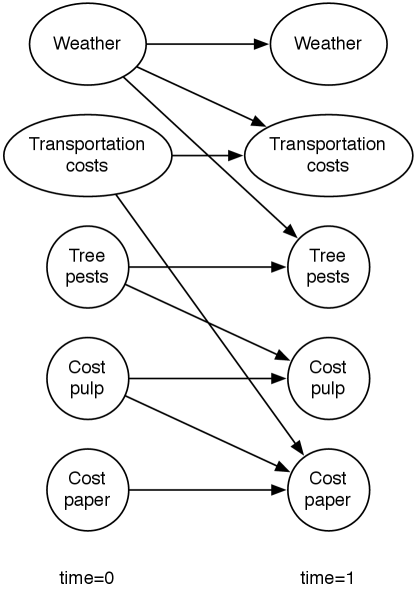
According to this figure, the variables are independent at time 0.
This two-stage dynamic belief network can be expanded into a regular dynamic belief network by replicating the nodes for each time step, and the parents for future steps are a copy of the parents for the time 1 variables.
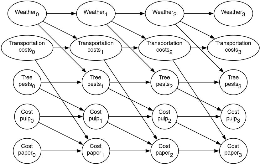
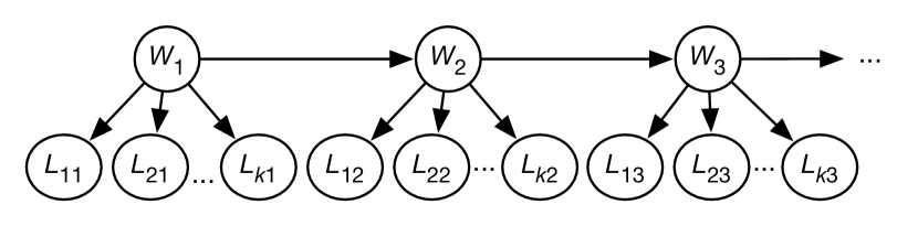
An expanded belief network for a horizon of 3 is shown in Figure 9.21. The subscripts represent the time that the variable is referring to.
9.6.5 Time Granularity
One of the problems with the definition of an HMM or a dynamic belief network is that the model depends on the time granularity. The time granularity specifies how often a dynamic system transitions from one state to the next. The time granularity could either be fixed, for example each day or each thirtieth of a second, or it could be event based, where a time step occurs when something interesting occurs. If the time granularity were to change, for example from daily to hourly, the conditional probabilities would also change.
One way to model the dynamics independently of the time granularity is to model continuous time, where for each variable and each value for the variable, the following are specified:
-
•
a distribution of how long the variable is expected to keep that value (e.g., an exponential decay) and
-
•
what value it will transition to when its value changes.
Given a discretization of time, where time moves from one state to the next in discrete steps, a dynamic belief network can be constructed from this information. If the discretization of time is fine enough, ignoring multiple value transitions in each time step will result only in small errors.
9.6.6 Probabilistic Language Models
Markov chains are the basis of simple language models, which have proved to be very useful in various natural language processing tasks in daily use.
Assume that a document is a sequence of sentences, where a sentence is a sequence of words. Consider the sorts of sentences that people may speak to a system or ask as a query to a help system. They may not be grammatical, and often contain words such as “thx” or “zzz”, which may not be typically thought of as words.
In the set-of-words model, a sentence (or a document) is treated as the set of words that appear in the sentence, ignoring the order of the words or whether the words are repeated. For example, the sentence “how can I phone my phone” would be treated as the set “can”, “how”, “I”, “my”, “phone”.
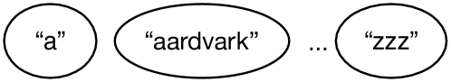
To represent the set-of-words model as a belief network, as in Figure 9.22, there is a Boolean random variable for each word. In this figure, the words are independent of each other (but they do not have to be). This belief network requires the probability of each word appearing in a sentence: , , …, . To condition on the sentence “how can I phone my phone”, all of the words in the sentence are assigned true, and all of the other words are assigned false. Words that are not defined in the model are either ignored, or are given a default (small) probability. The probability of sentence is .
A set-of-words model is not very useful by itself, but is often used as part of a larger model, as in the following example.
Example 9.36.
Suppose you want to develop a help system to determine which help page users are interested in based on the keywords they give in a query to a help system.
The system will observe the words that the user gives. Instead of modeling the sentence structure, assume that the set of words used in a query will be sufficient to determine the help page.
The aim is to determine which help page the user wants. Suppose that the user is interested in one and only one help page. Thus, it seems reasonable to have a node with domain the set of all help pages, .
One way this could be represented is as a naive Bayes classifier. A naive Bayes classifier is a belief network that has a single node – the class – that directly influences the other variables, and the other variables are independent of each other given the class. Figure 9.23 shows a naive Bayes classifier for the help system. The value of the class is the help page the user is interested in. The other nodes represent the words used in a query. This network embodies the independence assumption: the words used in a query depend on the help page the user is interested in, and the words are conditionally independent of each other given the help page.
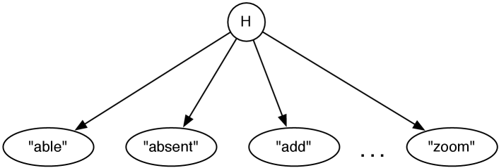
This network requires for each help page , which specifies how likely it is that a user would want this help page given no information. This network assumes the user is interested in exactly one help page, and so .
The network also requires, for each word and for each help page , the probability . These may seem more difficult to acquire but there are a few heuristics available. The sum of these values should be the average number of words in a query. We would expect words that appear in the help page to be more likely to be used when asking for that help page than words not in the help page. There may also be keywords associated with the page that may be more likely to be used. There may also be some words that are just used more, independently of the help page the user is interested in. Example 10.5 shows how to learn the probabilities of this network from experience.
To condition on the set of words in a query, the words that appear in the query are observed to be true and the words that are not in the query are observed to be false. For example, if the help text was “the zoom is absent”, the words “the”, “zoom”, “is”, and “absent” would be observed to be true, and the other words would be observed to be false. Once the posterior for has been computed, the most likely few help topics can be shown to the user.
Some words, such as “the” and “is”, may not be useful in that they have the same conditional probability for each help topic and so, perhaps, would be omitted from the model. Some words that may not be expected in a query could also be omitted from the model.
Note that the conditioning included the words that were not in the query. For example, if page was about printing problems, you might expect that people who wanted page would use the word “print”. The non-existence of the word “print” in a query is strong evidence that the user did not want page .
The independence of the words given the help page is a strong assumption. It probably does not apply to words like “not”, where which word “not” is associated with is very important. There may even be words that are complementary, in which case you would expect users to use one and not the other (e.g., “type” and “write”) and words you would expect to be used together (e.g., “go” and “to”); both of these cases violate the independence assumption. It is an empirical question as to how much violating the assumptions hurts the usefulness of the system.

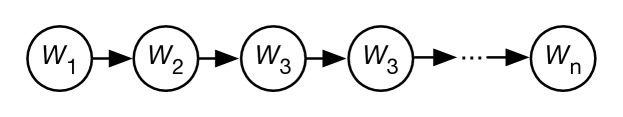
In a bag-of-words or unigram model, a sentence is treated as a bag (multi-set) of words, representing the number of times a word is used in a sentence, but not the order of the words. Figure 9.24 shows how to represent a unigram as a belief network. For the sequence of words, there is a variable for each position , with domain of each variable the set of all words, such as . The domain is often augmented with a symbol, “”, representing the end of the sentence, and with a symbol “?” representing a word that is not in the model.
To condition on the sentence “how can I phone my phone”, the word is observed to be “how”, the variable is observed to be “can”, etc. Word is assigned . Both and are assigned the value “phone”. There are no variables onwards.
The unigram model assumes a stationary distribution, where the prior distribution of is the same for each . The value of is the probability that a randomly chosen word is . More common words have a higher probability than less common words.
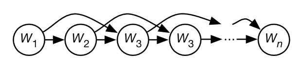
In a bigram model, the probability of each word depends on the previous word in the sentence. It is called a bigram model because it depends on pairs of words. Figure 9.25 shows the belief-network representation of a bigram model. This needs a specification of .
To make not be a special case, introduce a new word ; intuitively is the “word” between sentences. For example, is the probability that the word “cat” is the first word in a sentence. is the probability that the sentence ends after the word “cat”.
In a trigram model, each triple of words is modeled. This is represented as a belief network in Figure 9.26. This requires ; the probability of each word given the previous two words.
| the | 0.0464 |
| of | 0.0294 |
| and | 0.0228 |
| to | 0.0197 |
| in | 0.0156 |
| a | 0.0152 |
| is | 0.00851 |
| that | 0.00806 |
| for | 0.00658 |
| was | 0.00508 |
| same | 0.01023 |
| first | 0.00733 |
| other | 0.00594 |
| most | 0.00558 |
| world | 0.00428 |
| time | 0.00392 |
| two | 0.00273 |
| whole | 0.00197 |
| people | 0.00175 |
| great | 0.00102 |
| time | 0.15236 |
| as | 0.04638 |
| way | 0.04258 |
| thing | 0.02057 |
| year | 0.00989 |
| manner | 0.00793 |
| in | 0.00739 |
| day | 0.00705 |
| kind | 0.00656 |
| with | 0.00327 |
Unigram, bigram, and trigram probabilities derived from the Google books Ngram viewer (https://books.google.com/ngrams/) for the year 2000. is for the top 10 words, which are found by using the query “*” in the viewer. is part of a bigram model that represents for the top 10 words. This is derived from the query “the *” in the viewer. is part of a trigram model; the probabilities given represent , which is derived from the query “the same *” in the viewer.
In general, in an n-gram model, the probability of each word given the previous words is modeled. This requires considering each sequence of words, and so the complexity of representing this as a table grows with , where is the number of words. Figure 9.27 shows some common unigram, bigram, and trigram probabilities.
The conditional probabilities are typically not represented as tables, because the tables would be too large, and because it is difficult to assess the probability of a previously unknown word, or the probability of the next word given a previously unknown word or given an uncommon phrase. Instead, one could use context-specific independence, such as, for trigram models, represent the probability of the next word conditioned on some of the pairs of words, and if none of these hold, use , as in a bigram model. For example, the phrase “frightfully green” is not common, and so to compute the probability of the next word, , it is typical to use , which is easier to assess and learn.
Transformers, when used in generative language models, are n-gram models, where – the window size of the transformer – is very large (in GPT-3, is 2048). A neural network, using attention, gives the probability of the next word given the previous words in the window. Note that a transformer model used in an encoder to find a representation for a text uses the words after, as well as the words before, each word.
Any of these models could be used in the help system of Example 9.36, instead of the set-of-words model used there. These models may be combined to give more sophisticated models, as in the following example.
Example 9.37.
Consider the problem of spelling correction as users type into a phone’s onscreen keyboard to create sentences. Figure 9.28 gives a predictive typing model that does this (and more).
The variable is the th word in the sentence. The domain of each is the set of all words. This uses a bigram model for words, and assumes is provided as the language model. A stationary model is typically appropriate.
The variable represents the th letter in word . The domain of each is the set of characters that could be typed. This uses a unigram model for each letter given the word, but it would not be a stationary model, as for example the probability distribution of the first letter given the word “print” is different from the probability distribution of the second letter given the word “print”. We would expect to be close to 1 if the th letter of word is . The conditional probability could incorporate common misspellings and common typing errors (e.g., switching letters, or if someone tends to type slightly higher on the phone’s screen).
For example, would be close to 1, but not equal to 1, as the user could have mistyped. Similarly, would be high. The distribution for the second letter in the word, , could take into account mistyping adjacent letters (“e” and “t” are adjacent to “r” on the standard keyboard) and missing letters (maybe “i” is more likely because it is the third letter in “print”). In practice, these probabilities are typically extracted from data of people typing known sentences, without needing to model why the errors occurred.
The word model allows the system to predict the next word even if no letters have been typed. Then, as letters are typed, it predicts the word, based on the previous words and the typed letters, even if some of the letters are mistyped. For example, if the user types “I cannot pint”, it might be more likely that the last word is “print” than “pint” because of the way the model combines all of the evidence.
A topic model predicts the topics of a document from the sentences typed. Knowing the topic of a document helps people find the document or similar documents even if they do not know what words are in the document.
Example 9.38.
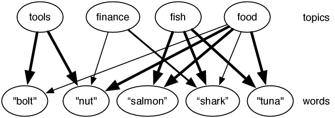
Figure 9.29 shows a simple topic model based on a set-of-words language model. There is a set of topics (four are given) which are a priori independent of each other. In this model, the words are independent of each other given the topic. A noisy-or is used to model how each word depends on the topics.
The noisy-or model can be represented by having a variable for each topic–word pair where the word is relevant for the topic. For example, the variable represents the probability that the word is in the document because the topic is . This variable has probability zero if the topic is not and has the probability that the word would appear when the topic is (and there are no other relevant topics). The word would appear, with probability 1 if is true or if an analogous variable, , is true, and with a small probability otherwise (the probability that it appears without one of the topics). Thus, each topic–word pair where the word is relevant to the topic is modeled by a single weight. In Figure 9.29, the higher weights are shown by thicker lines.
Given the words, the topic model is used to infer the distribution over topics. Once a number of words that are relevant to a topic are given, the topic becomes more likely, and so other words related to that topic also become more likely. Indexing documents by the topic lets us find relevant documents even if different words are used to look for a document.
This model is based on Google’s Rephil, which has 12,000,000 words (where common phrases are treated as words), a million topics and 350 million topic–word pairs with nonzero probability. In Rephil, the topics are structured hierarchically into a tree.
It is possible to mix these patterns, for example by using the current topics to predict the word in a predictive typing model with a topic model.
Models based on n-grams cannot represent all of the subtleties of natural language, as exemplified by the following example.
Example 9.39.
Consider the sentence
A tall person with a big hairy cat drank the cold milk.
In English, this is unambiguous; the person drank the milk. Consider how an n-gram might fare with such a sentence. The problem is that the subject (“person”) is far away from the verb (“drank”). It is also plausible that the cat drank the milk. It is easy to think of variants of this sentence where the word “person” is arbitrarily far away from the object of the sentence (“the cold milk”) and so would not be captured by any n-gram, unless was very large. Such sentences can be handled using a hidden state as in a long short-term memory (LSTM) or by explicitly building a parse tree, as described in Section 15.7.
Artificial Intelligence: Foundations of Computational Agents, Poole
& Mackworth
Copyright © 2023, David L. Poole and Alan K. Mackworth. 
This work is licensed under a Creative Commons Attribution-NonCommercial-NoDerivatives 4.0 International License.