10 Learning with Uncertainty 10.1 Probabilistic Learning 10.3 Unsupervised Learning

10.2 Bayesian Learning

Instead of just choosing the most likely hypothesis, it is typically more useful to use the posterior probability distribution of hypotheses, in what is called Bayesian learning.

Suppose $E$ is the set of training examples and a test example has inputs $X{\,{=}\,}x$ (written as $x$ ) and target $Y$ . The aim is to compute $P(Y\mid x\wedge E)$ . This is the probability distribution of the target variable given the particular inputs and the examples. The role of a model is to be the assumed generator of the examples. If $M$ is a set of disjoint and covering models:

$\displaystyle P(Y\mid x\wedge E)$	$\displaystyle\mbox{}=\sum_{m\in M}P(Y\wedge m\mid x\wedge E)$
	$\displaystyle\mbox{}=\sum_{m\in M}P(Y\mid m\wedge x\wedge E)*P(m\mid x\wedge E)$
	$\displaystyle\mbox{}=\sum_{m\in M}P(Y\mid m\wedge x)*P(m\mid E)~{}.$	(10.3)

The first two equalities follow from the definition of (conditional) probability. The last equality relies on two assumptions: the model includes all the information about the examples that is necessary for a particular prediction, $P(Y\mid m\wedge x\wedge E)=P(Y\mid m\wedge x)$ , and the model does not change depending on the inputs of the new example, $P(m\mid x\wedge E)=P(m\mid E)$ . Instead of choosing the best model, Bayesian learning relies on model averaging, averaging over the predictions of all the models, where each model is weighted by its posterior probability given the training examples, as in Equation 10.3.

$P(m\mid E)$ can be computed using Bayes’ rule (Equation 10.1), in terms of the prior $P(E)$ , the likelihood $P(E\mid m)$ , and a normalization term.

A common assumption is that examples $E=\{e_{1},\dots,e_{k}\}$ are independent and identically distributed (i.i.d.) given model $m$ , which means examples $e_{i}$ and $e_{j}$ , for $i\neq j$ , are independent given $m$ :

P(E\mid m)=\prod_{i=1}^{k}P(e_{i}\mid m)~{}.

The i.i.d. assumption can be represented as the belief network of Figure 10.1.

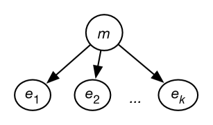
Refer to caption — Figure 10.1: The i.i.d. assumption as a belief network

A standard reasoning technique in such a network is to condition on the observed $e_{i}$ and to either query an unobserved $e_{j}$ variable, which provides a probabilistic prediction for unseen examples, or query $m$ , which provides a distribution over models.

The inference methods of the previous chapter could be used to compute the posterior probabilities. However, the exact methods presented are only applicable when $m$ is finite, because they involve enumerating the domains of the variables. However, $m$ is usually more complicated (often including real-valued components) than these exact techniques can handle, and approximation methods are required. For some cases, the inference can be exact using special-case algorithms.

The simplest case (Section 10.2.1) is to learn probabilities of a single discrete variable. Bayesian learning can also be used for learning decision trees (Section 10.2.3), learning the structure and probabilities of belief networks (Section 10.4), and more complicated cases.

10.2.1 Learning Probabilities

The simplest learning task is to learn a single Boolean random variable, $Y$ , with no input features, as in Section 7.2.2. The aim is to learn the posterior distribution of $Y$ conditioned on the training examples.

Example 10.1.

Consider the problem of predicting the next toss of a thumbtack (drawing pin), where the outcomes $T a i l s$ and $H e a d s$ are as follows:

Suppose you tossed a thumbtack a number of times and observed $E$ , a particular sequence of $n_{0}$ instances of $T a i l s$ and $n_{1}$ instances of $H e a d s$ . Assume the tosses are independent, and that $H e a d s$ occurs with probability $\phi$ . The likelihood is

P(E\mid\phi)=\phi^{n_{1}}*(1-\phi)^{n_{0}}.

This is a maximum when the log-likelihood

\log P(E\mid\phi)=n_{1}*\log\phi+n_{0}*\log(1-\phi)

is a maximum, and the negation of the average log-likelihood, the categorical log loss, is a minimum, which occur when $\phi=\frac{n_{1}}{n_{0}+n_{1}}$ .

Note that if $n_{1}=0$ , then $\phi$ is zero, which would indicate that $H e a d s$ is impossible; similarly, $n_{1}=0$ would predict that $T a i l s$ is impossible, which is an instance of overfitting. A MAP model would also take into account a prior.

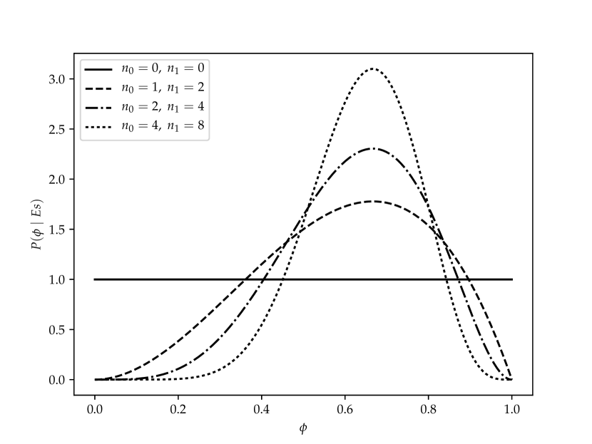
Reverend Thomas Bayes [1763] had the insight to treat a probability as a real-valued random variable. For a Boolean variable, $Y$ , a real-valued variable, $\phi$ , on the interval $[0,1]$ represents the probability of $Y$ . Thus, by definition of $\phi$ , $P(Y{\,{=}\,}true\mid\phi)=\phi$ and $P(Y{\,{=}\,}false\mid\phi)=1-\phi$ .

Suppose, initially, an agent considers all values in the interval $[0,1]$ equally likely to be the value of $\phi$ . This can be modeled with the variable $\phi$ having a uniform distribution over the interval $[0,1]$ . This is the probability density function labeled $n_{0}{\,{=}\,}0,n_{1}{\,{=}\,}0$ in Figure 10.2.

The probability distribution of $\phi$ is updated by conditioning on observed examples. Let the examples $E$ be the particular sequence of observations that resulted in $n_{1}$ occurrences of $Y{\,{=}\,}true$ and $n_{0}$ occurrences of $Y{\,{=}\,}false$ . Bayes’ rule and the i.i.d. assumption gives

	$\displaystyle P(\phi\mid E)$	$\displaystyle=\frac{P(E\mid\phi)*P(\phi)}{P(E)}$
		$\displaystyle\propto\phi^{n_{1}}(1-\phi)^{n_{0}}P(\phi).$

The denominator is a normalizing constant to ensure the area under the curve is 1.

Example 10.2.

Consider the thumbtack of Example 10.1 with a uniform prior.

With a uniform prior and no observations, shown as the $n_{0}=1,n_{1}=2$ line of Figure 10.2, the MAP estimate is undefined – every point is a maximum – and the expected value is 0.5.

When a single heads and no tails is observed, the distribution is a straight line from point $(0,0)$ to point $(1,2)$ . The most likely prediction – the MAP estimate – is $\phi=1$ . The expected value of the resulting distribution is $\phi=2/3$ .

When two heads and one tails are observed, the resulting distribution is the $n_{0}=1,n_{1}=2$ line of Figure 10.2. The mode is at $2/3$ and the expected value is $3/5$ .

Figure 10.2 gives some posterior distributions of the variable $\phi$ based on different sample sizes, given a uniform prior. The cases are $(n_{0}{\,{=}\,}1,n_{1}{\,{=}\,}2)$ , $(n_{0}{\,{=}\,}2,n_{1}{\,{=}\,}4)$ , and $(n_{0}{\,{=}\,}4,n_{1}{\,{=}\,}8)$ . Each of these peak at the same place, namely at $\frac{2}{3}$ . More training examples make the curve sharper.

When eight heads and four tails are observed, the mode is at $2/3$ and the expected value is $5/14$ . Notice how the expected value for this case is closer to the empirical proportion of heads in the training data than when $n_{0}=1,n_{1}=2$ , even though the modes are the same empirical proportion.

The distribution of this example is known as the beta distribution; it is parameterized by two counts, $\alpha_{0}$ and $\alpha_{1}$ , and a probability $\phi$ . Traditionally, the $\alpha_{i}$ parameters for the beta distribution are one more than the counts; thus, $\alpha_{i}=n_{i}+1$ . The beta distribution is

Beta^{\alpha_{0},\alpha_{1}}(\phi)=\frac{\phi^{\alpha_{1}-1}*(1-\phi)^{\alpha_% {0}-1}}{Z}

where $Z$ is a normalizing constant that ensures the integral over all values is 1. Thus, the uniform distribution on $[0,1]$ is the beta distribution $Beta^{1,1}$ .

The mode – the value with the maximum probability – of the beta distribution $Beta^{\alpha_{0},\alpha_{1}}$ is $\phi=\frac{\alpha_{0}-1}{\alpha_{0}+\alpha_{0}-2}$ .

The expected value of the beta distribution $Beta^{\alpha_{0},\alpha_{1}}$ is $\phi=\frac{\alpha_{0}}{\alpha_{0}+\alpha_{0}}$

Thus, the expectation of the beta distribution with a uniform prior gives Laplace smoothing. This shows that Laplace smoothing is optimal for the thought experiment where a probability was selected uniformly in [0,1], training and test data were generated using that probability, and evaluated on test data.

The prior does not need to be the uniform distribution. A common prior is to use a beta distribution for the prior of $\phi$ , such as

P(\phi)=\phi^{c_{1}-1}*(1-\phi)^{c_{0}-1}

corresponding to $c_{1}$ pseudo-examples with outcome true, and $c_{0}$ false pseudo-examples. In this case, the posterior probability given examples $E$ that consists of a particular sequence of $n_{0}$ false and $n_{1}$ true examples is

P(\phi\mid E)\propto\phi^{c_{1}+n_{1}-1}*(1-\phi)^{c_{0}+n_{0}-1}.

In this case, the MAP estimate for $\phi$ , the probability of true, is

p=\frac{c_{1}+n_{1}-1}{c_{0}+n_{0}+c_{1}+n_{1}-2}

and the expected value is

p=\frac{c_{1}+n_{1}}{c_{0}+n_{0}+c_{1}+n_{1}}.

This prior has the same form as the posterior; both are described in terms of a ration of counts. A prior that has the same form as a posterior is called a conjugate prior.

Note that $E$ is the particular sequence of observations made. If the observation was just that there were a total of $n_{0}$ occurrences of $Y=false$ and $n_{1}$ occurrences of $Y=true$ , you would get a different answer, because you would have to take into account all the possible sequences that could have given this count. This is known as the binomial distribution.

In addition to using the posterior distribution of $\phi$ to derive the expected value, it can be used to answer other questions such as: What is the probability that the posterior probability, $\phi$ , is in the range $[a,b]$ ? In other words, derive $P((\phi\geq a\wedge\phi\leq b)\mid E)$ . This is the problem that Bayes [1763] solved in his posthumously published paper. The solution published – although in much more cumbersome notation because calculus had not been invented when it was written – was

\frac{\int_{a}^{b}p^{n}*(1-p)^{m-n}}{\int_{0}^{1}p^{n}*(1-p)^{m-n}}~{}.

This kind of knowledge is used in poll surveys when it may be reported that a survey is correct with an error of at most $5\%$ , $19$ times out of $20$ , and in a probably approximately correct (PAC) estimate. It guarantees an error at most $\epsilon$ at least $1-\delta$ of the time as follows:

•

If an agent predicts $\frac{a+b}{2}$ , the midpoint of the range $[a,b]$ , it will have error less than or equal to $\epsilon=\frac{b-a}{2}$ , exactly when the hypothesis is in $[a,b]$ .
•

Let $\delta=1-P(\phi\geq a\wedge\phi\leq b\mid E)$ . Then $1-\delta$ is $P(\phi\geq a\wedge\phi\leq b\mid E)$ , so
•

choosing the midpoint will result in an error at most $\epsilon$ in $1-\delta$ of the time.

Hoeffding’s inequality gives worst-case results, whereas the Bayesian estimate gives the expected number. The worst case provides looser bounds than the expected case.

Categorical Variables

Suppose $Y$ is a categorical variable with $k$ possible values. A distribution over a categorical variable is called a multinomial distribution. The Dirichlet distribution is the generalization of the beta distribution to cover categorical variables. The Dirichlet distribution with two sorts of parameters, the “counts” $\alpha_{1},\dots,\alpha_{k}$ , and the probability parameters $p_{1},\dots,p_{k}$ , is

Dirichlet^{\alpha_{1},\dots,\alpha_{k}}(p_{1},\dots,p_{k})=\frac{\prod_{j=1}^{% k}p_{j}^{\alpha_{j}-1}}{Z}

where $p_{i}$ is the probability of the $i$ th outcome (and so $0\leq p_{i}\leq 1$ ) and $\alpha_{i}$ is a positive real number and $Z$ is a normalizing constant that ensures the integral over all the probability values is 1. You can think of $a_{i}$ as one more than the count of the $i$ th outcome, $\alpha_{i}=n_{i}+1$ . The Dirichlet distribution looks like Figure 10.2 along each dimension (i.e., as each $p_{j}$ varies between 0 and 1).

For the Dirichlet distribution, the expected value outcome $i$ (averaging over all $p_{j}$ ) is

\frac{\alpha_{i}}{\sum_{j}\alpha_{j}}~{}.

The reason that the $\alpha_{i}$ parameters are one more than the counts in the definitions of the beta and Dirichlet distributions is to make this formula simple.

Suppose an agent must predict a value for $Y$ with domain $\{y_{1},\dots,y_{k}\}$ , and there are no inputs. The agent starts with a positive pseudocount $c_{i}$ for each $y_{i}$ . These counts are chosen before the agent has seen any of the data. Suppose the agent observes training examples with $n_{i}$ data points having $Y{\,{=}\,}y_{i}$ . The probability of $Y$ is estimated using the expected value

P(Y{\,{=}\,}y_{i})=\frac{c_{i}+n_{i}}{\sum_{i^{\prime}}c_{i^{\prime}}+n_{i^{% \prime}}}.

When the dataset is empty (all $n_{i}=0$ ), the $c_{i}$ are used to estimate probabilities. An agent does not have to start with a uniform prior; it could start with any prior distribution. If the agent starts with a prior that is a Dirichlet distribution, its posterior will be a Dirichlet distribution.

Thus, the beta and Dirichlet distributions provide a justification for using pseudocounts for estimating probabilities. A pseudocount of 1 corresponds to Laplace smoothing.

Probabilities from Experts

The use of pseudocounts also gives us a way to combine expert knowledge and data. Often a single agent does not have good data but may have access to multiple experts who have varying levels of expertise and who give different probabilities.

There are a number of problems with obtaining probabilities from experts:

•

experts’ reluctance to give an exact probability value that cannot be refined
•

representing the uncertainty of a probability estimate
•

combining the estimates from multiple experts
•

combining expert opinion with actual data.

Rather than expecting experts to give probabilities, the experts can provide counts. Instead of giving a real number for the probability of $A$ , an expert gives a pair of numbers as $\left<n,m\right>$ that is interpreted as though the expert had observed $n$ occurrences of $A$ out of $m$ trials. Essentially, the experts provide not only a probability, but also an estimate of the size of the dataset on which their estimate is based.

The counts from different experts can be combined together by adding the components to give the pseudocounts for the system. You should not necessarily believe an expert’s sample size, as people are often overconfident in their abilities. Instead, the size can be estimated taking into account the experiences of the experts. Whereas the ratio between the counts reflects the probability, different levels of confidence are reflected in the absolute values. Consider different ways to represent the probability $2/3$ . The pair $\left<2,3\right>$ , with two positive examples out of three examples, reflects extremely low confidence that would quickly be dominated by data or other experts’ estimates. The pair $\left<20,30\right>$ reflects more confidence – a few examples would not change it much, but tens of examples would. Even hundreds of examples would have little effect on the prior counts of the pair $\left<2000,3000\right>$ . However, with millions of data points, even these prior counts would have little impact on the resulting probability estimate.

10.2.2 Probabilistic Classifiers

A Bayes classifier is a probabilistic model that is used for supervised learning. A Bayes classifier is based on the idea that the role of a class is to predict the values of features for members of that class. Examples are grouped in classes because they have common values for some of the features. The learning agent learns how the features depend on the class and uses that model to predict the classification of a new example.

The simplest case is the naive Bayes classifier, which makes the independence assumption that the input features are conditionally independent of each other given the classification. The independence of the naive Bayes classifier is embodied in a belief network where the features are the nodes, the target feature (the classification) has no parents, and the target feature is the only parent of each input feature. This belief network requires the probability distributions $P(Y)$ for the target feature, or class, $Y$ and $P(X_{i}\mid Y)$ for each input feature $X_{i}$ . For each example, the prediction is computed by conditioning on observed values for the input features and querying the classification. Multiple target variables can be modeled and learned separately.

Example 10.3.

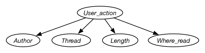
Suppose an agent wants to predict the user action given the data of Figure 7.1. For this example, the user action is the classification. The naive Bayes classifier for this example corresponds to the belief network of Figure 10.3. The input features form variables that are children of the classification.

The model of Figure 10.3 corresponds to $m$ in Figure 10.1.

Given an example with inputs $X_{1}{\,{=}\,}v_{1},\ldots,X_{k}{\,{=}\,}v_{k}$ , Bayes’ rule is used to compute the posterior probability distribution of the example’s classification, $Y$ :

	$\displaystyle P(Y\mid X_{1}$	$\displaystyle{\,{=}\,}v_{1},\ldots,X_{k}{\,{=}\,}v_{k})$
	$\displaystyle\mbox{}=\mbox{}$	$\displaystyle\frac{P(X_{1}{\,{=}\,}v_{1},\ldots,X_{k}{\,{=}\,}v_{k}\mid Y)*P(Y% )}{P(X_{1}{\,{=}\,}v_{1},\ldots,X_{k}{\,{=}\,}v_{k})}$
	$\displaystyle\mbox{}=\mbox{}$	$\displaystyle\frac{P(Y)\prod_{i=1}^{k}P(X_{i}{\,{=}\,}v_{i}\mid Y)}{\sum_{Y}P% (Y)\prod_{i=1}^{k}P(X_{i}{\,{=}\,}v_{i}\mid Y)}$

where the denominator is a normalizing constant to ensure the probabilities sum to 1.

Unlike many other models of supervised learning, the naive Bayes classifier can handle missing data where not all features are observed; the agent conditions on the features that are observed, which assumes the data is missing at random. Naive Bayes is optimal – it makes no independence assumptions beyond missing at random – if only a single $X_{i}$ is observed. As more of the $X_{i}$ are observed, the accuracy depends on how independent the $X_{i}$ are given $Y$ .

If $Y$ is Boolean and every $X_{i}$ is observed, naive Bayes is isomorphic to a logistic regression model; see page 9.3.3 for a derivation. They have identical predictions when the logistic regression weight for $X_{i}$ is the logarithm of the likelihood ratio, $\log P(X_{i}\mid h)/P(X_{i}\mid\neg h)$ . They are typically learned differently – but don’t need to be – with logistic regression trained to minimize log loss and naive Bayes trained for the conditional probabilities to be the MAP model or the expected value, given a prior.

To learn a classifier, the distributions of $P(Y)$ and $P(X_{i}\mid Y)$ for each input feature can be learned from the data. Each conditional probability distribution $P(X_{i}\mid Y)$ may be treated as a separate learning problem for each value of $Y$ , for example using beta or Dirichlet distributions.

Example 10.4.

Suppose an agent wants to predict the user action given the data of Figure 7.1. For this example, the user action is the classification. The naive Bayes classifier for this example corresponds to the belief network of Figure 10.3. The training examples are used to determine the probabilities required for the belief network.

Suppose the agent uses the empirical frequencies as the probabilities for this example. (Thus, it is not using any pseudocounts.) The maximum likelihood probabilities that can be derived from these data are

P(User\_action{\,{=}\,}reads)=\ifrac{9}{18}=0.5

P(Author{\,{=}\,}known\mid User\_action{\,{=}\,}reads)=\ifrac{2}{3}

P(Author{\,{=}\,}known\mid User\_action{\,{=}\,}skips)=\ifrac{2}{3}

P(Thread{\,{=}\,}new\mid User\_action{\,{=}\,}reads)=\ifrac{7}{9}

P(Thread{\,{=}\,}new\mid User\_action{\,{=}\,}skips)=\ifrac{1}{3}

P(Length{\,{=}\,}long\mid User\_action{\,{=}\,}reads)=0

P(Length{\,{=}\,}long\mid User\_action{\,{=}\,}skips)=\ifrac{7}{9}

P(Where\_read{\,{=}\,}home\mid User\_action{\,{=}\,}reads)=\ifrac{4}{9}

P(Where\_read{\,{=}\,}home\mid User\_action{\,{=}\,}skips)=\ifrac{4}{9}~{}.

Based on these probabilities, the features $A u t h o r$ and $Where\_read$ have no predictive power because knowing either does not change the probability that the user will read the article.

If the maximum likelihood probabilities are used, some conditional probabilities may be zero. This means that some features become predictive: knowing just one feature value can rule out a category. It is possible that some combinations of observations are impossible, and the classifier will have a divide-by-zero error if these are observed. See Exercise 10.1. This is a problem not necessarily with using a Bayes classifier, but rather with using empirical frequencies as probabilities.

The alternative to using the empirical frequencies is to incorporate pseudocounts. Pseudocounts can be engineered to have desirable behavior, before any data is observed and as more data is acquired.

Example 10.5.

Consider how to learn the probabilities for the help system of Example 9.36, where a helping agent infers what help page a user is interested in based on the words in the user’s query to the help system. Let’s treat the query as a set of words.

The learner must learn $P(H)$ . It could start with a pseudocount for each $h_{i}$ . Pages that are a priori more likely should have a higher pseudocount.

Similarly, the learner needs the probability $P(w_{j}\mid h_{i})$ , the probability that word $w_{j}$ will be used given the help page is $h_{i}$ . Because you may want the system to work even before it has received any data, the prior for these probabilities should be carefully designed, taking into account the frequency of words in the language, the words in the help page itself, and other information obtained by experience with other (help) systems.

Assume the following positive counts, which are observed counts plus suitable pseudocounts:

•

$c_{i}$ the number of times $h_{i}$ was the correct help page
•

$s=\sum_{i}c_{i}$ the total count
•

$u_{ij}$ the number of times $h_{i}$ was the correct help page and word $w_{j}$ was used in the query.

From these counts an agent can estimate the required probabilities

	$\displaystyle P(h_{i})$	$\displaystyle=c_{i}/s$
	$\displaystyle P(w_{j}\mid h_{i})$	$\displaystyle=u_{ij}/c_{i}$

from which $P(H\mid q)$ , the posterior distribution of help pages conditioned on the set of words $q$ in a user’s query, can be computed; see Example 10.3. It is necessary to use the words not in the query as well as the words in the query. For example, if a help page is about printing, the work “print” may be very likely to be used. The fact that “print” is not in a query is strong evidence that this is not the appropriate help page.

The system could present the help page(s) with the highest probability given the query.

When a user claims to have found the appropriate help page, the counts for that page and the words in the query are updated. Thus, if the user indicates that $h_{i}$ is the correct page, the counts $s$ and $c_{i}$ are incremented, and for each word $w_{j}$ used in the query, $u_{ij}$ is incremented. This model does not use information about the wrong page. If the user claims that a page is not the correct page, this information is not used.

The biggest challenge in building such a help system is not in the learning but in acquiring useful data. In particular, users may not know whether they have found the page they were looking for. Thus, users may not know when to stop and provide the feedback from which the system learns. Some users may never be satisfied with a page. Indeed, there may not exist a page they are satisfied with, but that information never gets fed back to the learner. Alternatively, some users may indicate they have found the page they were looking for, even though there may be another page that was more appropriate. In the latter case, the correct page may end up with its counts so low, it is never discovered. See Exercise 10.2.

Although there are some cases where the naive Bayes classifier does not produce good results, it is extremely simple, easy to implement, and often works very well. It is a good method to try for a new problem.

In general, the naive Bayes classifier works well when the independence assumption is appropriate, that is, when the class is a good predictor of the other features and the other features are independent given the class. This may be appropriate for natural kinds, where the classes have evolved because they are useful in distinguishing the objects that humans want to distinguish. Natural kinds are often associated with nouns, such as the class of dogs or the class of chairs.

The naive Bayes classifier can be expanded in a number of ways:

•

Some input features could be parents of the classification and some be children. The probability of the classification given its parents could be represented as a decision tree or a squashed linear function or a neural network.
•

The children of the classification do not have to be modeled as independent. In a tree-augmented naive Bayes (TAN) network, the children of the class variable are allowed to have zero or one other parents as long as the resulting graph is acyclic. This allows for a simple model that accounts for interdependencies among the children, while retaining efficient inference, as the tree structured in the children has a small treewidth.
•

Structure can be incorporated into the class variable. A latent tree model decomposes the class variable into a number of latent variables that are connected together in a tree structure. Each observed variable is a child of one of the latent variables. The latent variables allow a model of the dependence between the observed variables.

10.2.3 Probabilistic Learning of Decision Trees

The previous examples did not need the prior on the structure of models, as all the models were equally complex. However, learning decision trees requires a bias, typically in favor of smaller decision trees. The prior probability provides this bias.

If there are no examples with the same values for the input features but different values for the target feature, there are always multiple decision trees that fit the data perfectly. For every assignment of values that did not appear in the training set, there are decision trees that perfectly fit the training set, and make opposite predictions on the unseen examples. See the no-free-lunch theorem. If there is a possibility of noise, none of the trees that perfectly fit the training set may be the best model.

Example 10.6.

Consider the data of Figure 7.1, where the learner is required to predict the user’s actions.

One possible decision tree is the one given on the left of Figure 7.8. Call this decision tree $d_{2}$ ; the subscript being the depth. The likelihood of the data is $P(E\mid d_{2})=1$ . That is, $d_{2}$ accurately fits the data.

Another possible decision tree is the one with no internal nodes, and a single leaf that predicts $r e a d s$ with probability $\frac{1}{2}$ . This is the most likely tree with no internal nodes, given the data. Call this decision tree $d_{0}$ . The likelihood of the data given this model is

P(E\mid d_{0})=\left(\frac{1}{2}\right)^{9}*\left(\frac{1}{2}\right)^{9}% \approx 1.5*10^{-6}.

Another possible decision tree is one on the right of Figure 7.8, with one split on $L e n g t h$ and with probabilities on the leaves given by $P(reads\mid Length{\,{=}\,}long)=0$ and $P(reads\mid Length{\,{=}\,}short)=\frac{9}{11}$ . Note that $\frac{9}{11}$ is the empirical frequency of $r e a d s$ among the training set with $Length{\,{=}\,}short$ . Call this decision tree $d_{1a}$ . The likelihood of the data given this model is

P(E\mid d_{1a})=1^{7}*\left(\frac{9}{11}\right)^{9}*\left(\frac{2}{11}\right)^% {2}\approx 0.0543.

These are just three of the possible decision trees. Which is best depends on the prior on trees. The likelihood of the data is multiplied by the prior probability of the decision trees to determine the posterior probability of the decision tree.

10.2.4 Description Length

To find a most likely model $m$ given examples $E s$ – a model that maximizes $P(m\mid Es)$ – you can apply Bayes’ rule, ignore the denominator (which doesn’t depend on $m$ ), and so maximize $P(E\mid m)*P(m)$ ; see Formula 10.2. Taking the negative of the logarithm (base 2), means you can minimize

-\log_{2}P(E\mid m)-\log_{2}P(m).

This can be interpreted in terms of information theory. The term $-\log_{2}P(E\mid m)$ is the number of bits it takes to describe the data given the model $m$ . The term $-\log_{2}P(m)$ is the number of bits it takes to describe the model. A model that minimizes this sum is a minimum description length (MDL) model. The MDL principle is to choose the model that minimizes the number of bits it takes to describe both the model and the data given the model.

One way to think about the MDL principle is that the aim is to communicate the data as succinctly as possible. To communicate the data, first communicate the model, then communicate the data in terms of the model. The number of bits it takes to communicate the data using a model is the number of bits it takes to communicate the model plus the number of bits it takes to communicate the data in terms of the model.

As the logarithm function is monotonically increasing, the MAP model is the same as the MDL model. Choosing a model with the highest posterior probability is the same as choosing a model with a minimum description length.

The description length provides common units for probabilities and model complexity; they can both be described in terms of bits.

Example 10.7.

In Example 10.6, the definition of the priors on decision trees was left unspecified. The notion of a description length provides a basis for assigning priors to decision trees.

One code for a tree for a Boolean output with Boolean input features might be as follows. A decision tree is either 0 followed by a fixed-length probability, or 1 followed by a bit string representing a condition (an input feature) followed by the tree when the condition is false followed by the tree for when the condition is true. The condition might take $\lceil\log_{2}m\rceil$ , where $m$ is the number of input features. The probability could either be a fixed-length bit string, or depend on the data (see below). See Exercise 10.8.

It is often useful to approximate the description length of the model. One way to approximate the description length is to consider just representing the probabilistic parameters of the model. Let $|t|$ be the number of probabilistic parameters of the model $t$ . For a decision tree with probabilities at the leaves, $|t|$ is the number of leaves. For a linear function or a neural network, $|t|$ is the number of numerical parameters.

Suppose $|E|$ is the number of training examples. There are at most $|E|+1$ different probabilities the model needs to distinguish, because that probability is derived from the counts, and there can be from 0 to $|E|$ examples with a particular value true in the dataset. It takes $\log_{2}(|E|+1)\approx\log_{2}(|E|)$ bits to distinguish these probabilities. Thus, the problem of finding the MDL model can be approximated by minimizing

-\log_{2}P(E\mid t)+|t|*\log_{2}(|E|).

This value is the Bayesian information criteria (BIC) score.

Artificial Intelligence 3E