Artificial
Intelligence 3E
foundations of computational agents
9.7 Stochastic Simulation
Many problems are too big for exact inference, so one must resort to approximate inference. Some of the most effective methods are based on generating random samples from the (posterior) distribution that the network specifies.
Stochastic simulation is a class of algorithms based on the idea that a set of samples can be mapped to and from probabilities. For example, the probability means that out of 1000 samples, about 140 will have true. Inference can be carried out by going from probabilities into samples and from samples into probabilities.
The following sections consider three problems:
-
•
how to generate samples
-
•
how to infer probabilities from samples
-
•
how to incorporate observations.
These form the basis for methods that use sampling to compute the posterior distribution of a variable in a belief network, including rejection sampling, importance sampling, particle filtering, and Markov chain Monte Carlo.
9.7.1 Sampling from a Single Variable
The simplest case is to generate the probability distribution of a single variable. This is the base case the other methods build on.
From Probabilities to Samples
To generate samples from a single discrete or real-valued variable, , first totally order the values in the domain of . For discrete variables, if there is no natural order, just create an arbitrary ordering. Given this ordering, the cumulative probability distribution is a function of , defined by .
To generate a random sample for , select a random number in the domain . We select from a uniform distribution to ensure that each number between 0 and 1 has the same chance of being chosen. Let be the value of that maps to in the cumulative probability distribution. That is, is the element of such that or, equivalently, . Then, is a random sample of , chosen according to the distribution of .
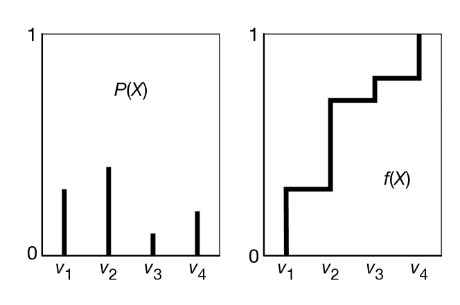
Example 9.40.
Consider a random variable with domain . Suppose , , , and . First, totally order the values, say . Figure 9.30 shows , the distribution for , and , the cumulative distribution for . Consider value ; 0.3 of the domain of maps back to . Thus, if a sample is uniformly selected from the -axis, has a 0.3 chance of being selected, has a chance of being selected, and so forth.
From Samples to Probabilities
Probabilities can be estimated from a set of samples using the sample average. The sample average of a proposition is the number of samples where is true divided by the total number of samples. The sample average approaches the true probability as the number of samples approaches infinity by the law of large numbers.
Hoeffding’s inequality provides an estimate of the error of the sample average, , given independent samples compared to the true probability, . means that the error is larger than , for .
Proposition 9.3 (Hoeffding).
Suppose is the true probability, and is the sample average from independent samples; then
This theorem can be used to determine how many samples are required to guarantee a probably approximately correct (PAC) estimate of the probability. To guarantee that the error is always less than some , infinitely many samples are required. However, if you are willing to have an error greater than in of the cases, solve for , which gives
For example, suppose you want an error less than , 19 times out of 20; that is, you are only willing to tolerate an error bigger than 0.1 in less than 5% of the cases. You can use Hoeffding’s bound by setting to and to , which gives . The following table gives some required number of examples for various combinations of values for and :
| 0.1 | 0.05 | 185 |
| 0.01 | 0.05 | 18445 |
| 0.1 | 0.01 | 265 |
| 0.01 | 0.01 | 26492 |
Notice that many more examples are required to get accurate probabilities (small ) than are required to get good approximations (small ).
9.7.2 Forward Sampling
Using the cumulative distribution to generate samples only works for a single dimension, because all of the values must be put in a total order. Sampling from a distribution defined by multiple variables is difficult in general, but is straightforward when the distribution is defined using a belief network.
Forward sampling is a way to generate a sample of every variable in a belief network so that each sample is generated in proportion to its probability. This enables us to estimate the prior probability of any variable.
Suppose is a total ordering of the variables so that the parents of each variable come before the variable in the total order. Forward sampling draws a sample of all of the variables by drawing a sample of each variable in order. First, it samples using the cumulative distribution, as described above. For each of the other variables, due to the total ordering of variables, when it comes time to sample , it already has values for all of the parents of . It now samples a value for from the distribution of given the values already assigned to the parents of . Repeating this for every variable generates a sample containing values for all of the variables. The probability distribution of a query variable is estimated by considering the proportion of the samples that have assigned each value of the variable.
Example 9.41.
To create a set of samples for the belief network of Figure 9.3, suppose the variables are ordered: , , , , , .
| Sample | Tampering | Fire | Alarm | Smoke | Leaving | Report |
|---|---|---|---|---|---|---|
| false | true | true | true | false | false | |
| false | false | false | false | false | false | |
| false | true | true | true | true | true | |
| false | false | false | false | false | true | |
| false | false | false | false | false | false | |
| false | false | false | false | false | false | |
| true | false | false | true | true | true | |
| true | false | false | false | false | true | |
| … | ||||||
| true | false | true | true | false | false |
First the algorithm samples , using the cumulative distribution. Suppose it selects . Then it samples using the same method. Suppose it selects . Then it samples a value for , using the distribution . Suppose it selects . Next, it samples a value for using . And so on for the other variables. It has thus selected a value for each variable and created the first sample of Figure 9.31. Notice that it has selected a very unlikely combination of values. This does not happen very often; it happens in proportion to how likely the sample is. It repeats this until it has enough samples. In Figure 9.31, it generated 1000 samples.
The probability that is estimated from the proportion of the samples where the variable has value true.
Forward sampling is used in (large) language models, to generate text. A neural network, such as an LSTM or transformer, is used to represent the probability of the next word given the previous words. Forward sampling then generates a sample of text. Different runs produce different text, with a very low probability of repeating the same text. Forward sampling is also used in game playing, where it can be used to predict the distribution of outcomes of a game from a game position, given a probability distribution of the actions from a position, in what is called Monte Carlo tree search; see Section 14.7.3.
9.7.3 Rejection Sampling
Given some evidence , rejection sampling estimates using the formula
This is computed by considering only the samples where is true and by determining the proportion of these in which is true. The idea of rejection sampling is that samples are generated as before, but any sample where is false is rejected. The proportion of the remaining, non-rejected, samples where is true is an estimate of . If the evidence is a conjunction of assignments of values to variables, a sample is rejected when any variable is assigned a value different from its observed value.
| Sample | Tampering | Fire | Alarm | Smoke | Leaving | Report | |
|---|---|---|---|---|---|---|---|
| false | false | true | false | ✘ | |||
| false | true | false | true | false | false | ✔ | |
| false | true | true | false | ✘ | |||
| false | true | false | true | false | false | ✔ | |
| false | true | true | true | true | true | ✘ | |
| false | false | false | true | false | false | ✔ | |
| true | false | false | false | ✘ | |||
| true | true | true | true | true | true | ✘ | |
| … | |||||||
| true | false | true | false | ✘ |
Example 9.42.
Figure 9.32 shows how rejection sampling is used to estimate . Any sample with is rejected. The sample is rejected without considering any more variables. Any sample with is rejected. The sample average from the remaining samples (those marked with ✔) is used to estimate the posterior probability of .
Because , we would expect about 13 samples out of the 1000 to have true; the other 987 samples would have false, and so would be rejected. Thus, 13 is used as in Hoeffding’s inequality, which, for example, guarantees an error for any probability computed from these samples of less than in about 86% of the cases, which is not very accurate.
The error in the probability of depends on the number of samples that are not rejected, which is proportional to . Hoeffding’s inequality can be used to estimate the error of rejection sampling, where is the number of non-rejected samples. Therefore, the error depends on .
Rejection sampling does not work well when the evidence is unlikely. This may not seem like that much of a problem because, by definition, unlikely evidence is unlikely to occur. But, although this may be true for simple models, for complicated models with complex observations, every possible observation may be unlikely. Also, for many applications, such as in diagnosis, the user is interested in determining the probabilities because unusual observations are involved.
9.7.4 Likelihood Weighting
Instead of creating a sample and then rejecting it, it is possible to mix sampling with inference to reason about the probability that a sample would be rejected. In importance sampling methods, each sample has a weight, and the sample average uses the weighted average. Likelihood weighting is a simple form where the variables are sampled in the order defined by a belief network, and evidence is used to update the weights. The weights reflect the probability that a sample would not be rejected. More general forms of importance sampling are explored in Section 9.7.5.
Example 9.43.
Consider the belief network of Figure 9.3. In this , , and . Suppose is observed, and another descendant of is queried.
Starting with 1000 samples, approximately 10 will have , and the other 990 samples will have . In rejection sampling, of the 990 with , 1%, which is approximately 10, will have and so will not be rejected. The remaining 980 samples will be rejected. Of the 10 with , about 9 will not be rejected. Thus, about 98% of the samples are rejected.
In likelihood weighing, instead of sampling and rejecting most samples, the samples with are weighted by and the samples with are weighted with . This potentially give a much better estimate of any of the probabilities that use these samples.
Figure 9.33 shows the details of the likelihood weighting for computing for query variable and evidence . The loop (from line 15) creates a sample containing a value for all of the variables. Each observed variable changes the weight of the sample by multiplying by the probability of the observed value given the assignment of the parents in the sample. The variables not observed are sampled according to the probability of the variable given its parents in the sample. Note that the variables are sampled in an order to ensure that the parents of a variable have been assigned in the sample before the variable is selected.
To extract the distribution of the query variable , the algorithm maintains an array , such that is the sum of the weights of the samples where . This algorithm can also be adapted to the case where the query is some complicated condition on the values by counting the cases where the condition is true and those where the condition is false.
Example 9.44.
Consider using likelihood weighting to compute .
The following table gives a few samples. In this table, is the sample; is . The weight is , which is equal to , where the values for and are from the sample.
| Tampering | Fire | Alarm | Smoke | Leaving | Report | Weight |
|---|---|---|---|---|---|---|
| false | true | false | true | true | false | |
| true | true | true | true | false | false | |
| false | false | false | true | true | false | |
| false | true | false | true | false | false |
is estimated from the weighted proportion of the samples that have true.
9.7.5 Importance Sampling
Likelihood weighting is an instance of importance sampling. Importance samplingin general has:
-
•
Samples are weighted.
-
•
The samples do not need to come from the actual distribution, but can be from (almost) any distribution, with the weights adjusted to reflect the difference between the distributions.
-
•
Some variables can be summed out and some sampled.
This freedom to sample from a different distribution allows the algorithm to choose better sampling distributions to give better estimates.
Stochastic simulation can be used to compute the expected value of real-valued variable under probability distribution using
where is a sample that is sampled with probability , and is the number of samples. The estimate gets more accurate as the number of samples grows.
Suppose it is difficult to sample with the distribution , but it is easy to sample from a distribution . We adapt the previous equation to estimate the expected value from , by sampling from using
where the last sum is over samples selected according to the distribution . The distribution is called a proposal distribution. The only restriction on is that it should not be zero for any cases where is not zero (i.e., if then ).
Recall that for Boolean variables, with true represented as 1 and false as 0, the expected value is the probability. So the methods here can be used to compute probabilities.
The algorithm of Figure 9.33 can be adapted to use a proposal distribution as follows: in line 20, it should sample from , and in a new line after that, it updates the value of by multiplying it by .
Example 9.45.
In the running alarm example, . As explained in Example 9.43, if the algorithm samples according to the prior probability, would only be true in about 19 samples out of 1000. Likelihood weighting ended up with a few samples with high weights and many samples with low weights, even though the samples represented similar numbers of cases.
Suppose, instead of sampling according to the probability, the proposal distribution with is used. Then is sampled 50% of the time. According to the model , thus each sample with is weighted by and each sample with is weighted by .
With importance sampling with as the proposal distribution, half of the samples will have , and the model specifies . Given the evidence , these will be weighted by . The other half of the samples will have , and the model specifies . These samples will have a weighting of . Notice how all of the samples have weights of the same order of magnitude. This means that the estimates from these are much more accurate.
Importance sampling can also be combined with exact inference. Not all variables need to be sampled. The variables not sampled can be summed out by variable elimination.
The best proposal distribution is one where the samples have approximately equal weight. This occurs when sampling from the posterior distribution. In adaptive importance sampling, the proposal distribution is modified to approximate the posterior probability of the variable being sampled.
9.7.6 Particle Filtering
Importance sampling enumerates the samples one at a time and, for each sample, assigns a value to each variable. It is also possible to start with all of the samples and, for each variable, generate a value for that variable for each sample. For example, for the data of Figure 9.31, the same data could be generated by generating all of the samples for before generating the samples for . The particle filtering algorithm or sequential Monte Carlo (SMC) generates all the samples for one variable before moving to the next variable. It does one sweep through the variables, and for each variable it does a sweep through all of the samples. This algorithm is advantageous when variables are generated dynamically and when there are unboundedly many variables, as in the sequential models. It also allows for a new operation of resampling.
In particle filtering, the samples are called particles. A particle is a - dictionary, where a dictionary is a representation of a partial function from keys into values; here the key is a variable and the particle maps to its value. A particle has an associated weight. A set of particles is a population.
The algorithm starts with a population of empty dictionaries. The algorithm repeatedly selects a variable according to an ordering where a variable is selected after its parents. If the variable is not observed, for each particle, a value for the variable for that particle is sampled from the distribution of the variable given the assignment of the particle. If the variable is observed, each particle’s weight is updated by multiplying by the probability of the observation given the assignment of the particle.
Given a population of particles, resampling generates a new population of particles, each with the same weight. Each particle is selected with probability proportional to its weight. Resampling can be implemented in the same way that random samples for a single random variable are generated, but particles, rather than values, are selected. Some particles may be selected multiple times and others might not be selected at all.
The particle filtering algorithm is shown in Figure 9.34. Line 16 assigns its observed value. Line 17, which is used when is observed, updates the weights of the particles according to the probability of the observation on . Line 22 assigns a value sampled from the distribution of given the values of its parents in the particle.
This algorithm resamples after each observation. It is also possible to resample less often, for example, after a number of variables are observed.
Importance sampling is equivalent to particle filtering without resampling. The principal difference is the order in which the particles are generated. In particle filtering, each variable is sampled for all particles, whereas, in importance sampling, each particle (sample) is sampled for all variables before the next particle is considered.
Particle filtering has two main advantages over importance sampling. First, it can be used for an unbounded number of variables, as in hidden Markov models and dynamic belief networks. Second, resampling enables the particles to better cover the distribution over the variables. Whereas importance sampling will result in some particles that have very low probability, with only a few of the particles covering most of the probability mass, resampling lets many particles more uniformly cover the probability mass.
Example 9.46.
Consider using particle filtering to compute for the belief network of Figure 9.3. First generate the particles . Suppose it first samples . Out of the 1000 particles, about 10 will have and about 990 will have (as ). It then absorbs the evidence . Those particles with will be weighted by 0.9 as and those particles with will be weighted by 0.01 as . It then resamples; each particle is chosen in proportion to its weight. The particles with will be chosen in the ratio . Thus, about 524 particles will be chosen with , and the remainder with . The other variables are sampled, in turn, until is observed, and the particles are resampled. At this stage, the probability of will be the proportion of the samples with tampering being true.
Note that in particle filtering the particles are not independent, so Hoeffding’s inequality is not directly applicable.
9.7.7 Markov Chain Monte Carlo
The previously described methods went forward through the network (parents were sampled before children), and were not good at passing information back through the network. The method described in this section can sample variables in any order.
A stationary distribution of a Markov chain is a distribution of its variables that is not changed by the transition function of the Markov chain. If the Markov chain mixes enough, there is a unique stationary distribution, which can be approached by running the Markov chain long enough. The idea behind Markov chain Monte Carlo (MCMC) methods to generate samples from a distribution (e.g., the posterior distribution given a belief network) is to construct a Markov chain with the desired distribution as its (unique) stationary distribution and then sample from the Markov chain; these samples will be distributed according to the desired distribution. The first few samples are typically discarded in a burn-in period, as these samples may be far from the stationary distribution.
One way to create a Markov chain from a belief network with observations, is to use Gibbs sampling. The idea is to clamp observed variables to the values they were observed to have, and sample the other variables. Each variable is sampled from the distribution of the variable given the current values of the other variables. Note that each variable only depends on the values of the variables in its Markov blanket. The Markov blanket of a variable in a belief network contains ’s parents, ’s children, and the other parents of ’s children; these are all of the variables that appear in factors with .
Figure 9.35 gives pseudocode for Gibbs sampling. The only part not defined is how to randomly sample from . This can be computed by noticing that for each value of , the probability is proportional to the product of the values of the factors in which appears projected onto the current value of all of the other variables.
Example 9.47.
Consider using particle filtering to compute for the belief network of Figure 9.3. Figure 9.36 shows a sequence of samples, where the underlined value is selected at each step.
| Sample | Tampering | Fire | Alarm | Smoke | Leaving | Report |
|---|---|---|---|---|---|---|
| true | true | false | true | false | false | |
| true | true | false | true | false | false | |
| true | true | false | true | false | false | |
| true | true | true | true | false | false | |
| true | true | true | true | true | false | |
| false | true | true | true | true | false | |
| … | ||||||
| false | true | true | true | true | false |
and are clamped at true and false, respectively.
Sample is generated at random and the variable is selected. and form the Markov blanket for , so a random sample for is drawn; suppose it is true. This gives sample .
Given , a random value from is drawn. Suppose it is true. This gives sample . Next a random value from is drawn; suppose it is true.
At the end, the estimate of probability of is the proportion of true cases in the samples after the burn-in period.
Gibbs sampling will approach the correct probabilities as long as there are no zero probabilities. How quickly it approaches the distribution depends on how quickly the probabilities mix (how much of the probability space is explored), which depends on how extreme the probabilities are. Gibbs sampling works well when the probabilities are not extreme (very close to 0 or 1).
Example 9.48.
As a problematic case for Gibbs sampling, consider a simple example with three Boolean variables , , and , with as the parent of , and as the parent of . Suppose , , , , and . There are no observations and the query variable is . The two assignments with all variables having the same value are equally likely and are much more likely than the other assignments. Gibbs sampling will quickly get to one of these assignments, and will take a long time to transition to the other assignments (as it requires some very unlikely choices). If 0.99 and 0.01 were replaced by numbers closer to 1 and 0, it would take even longer to converge.
Artificial Intelligence: Foundations of Computational Agents, Poole
& Mackworth
Copyright © 2023, David L. Poole and Alan K. Mackworth. 
This work is licensed under a Creative Commons Attribution-NonCommercial-NoDerivatives 4.0 International License.