9 Reasoning with Uncertainty 9 Reasoning with Uncertainty 9.2 Independence

9.1 Probability

To make a good decision, an agent cannot simply assume what the world is like and act according to that assumption. It must consider multiple hypotheses when making a decision, and not just act on the most likely prediction. Consider the following example.

Example 9.1.

Many people consider it sensible to wear a seat belt when traveling in a car because, in an accident, wearing a seat belt reduces the risk of serious injury. However, consider an agent that commits to assumptions and bases its decision on these assumptions. If the agent assumes it will not have an accident, it will not bother with the inconvenience of wearing a seat belt. If it assumes it will have an accident, it will not go out. In neither case would it wear a seat belt! A more intelligent agent may wear a seat belt because the inconvenience of wearing a seat belt is far outweighed by the increased risk of injury or death if it has an accident. It does not stay at home too worried about an accident to go out; the benefits of being mobile, even with the risk of an accident, outweigh the benefits of the extremely cautious approach of never going out. The decisions of whether to go out and whether to wear a seat belt depend on the likelihood of having an accident, how much a seat belt helps in an accident, the inconvenience of wearing a seat belt, and how important it is to go out. The various trade-offs may be different for different agents. Some people do not wear seat belts, and some people do not go in cars because of the risk of accident.

Reasoning with uncertainty has been studied in the fields of probability theory and decision theory. Probability is the calculus needed for gambling. When an agent makes decisions and is uncertain about the outcomes of its actions, it is gambling on the outcomes. However, unlike a gambler at the casino, an agent that has to survive in the real world cannot opt out and decide not to gamble; whatever it does – including doing nothing – involves uncertainty and risk. If it does not take the probabilities of possible outcomes into account, it will eventually lose at gambling to an agent that does. This does not mean, however, that making the best decision guarantees a win.

Probability is the calculus of belief; probability theory tells us how to update beliefs based on new information. When an agent doesn’t have any information about the particular situation; it will still have beliefs. The belief of an agent before it observes anything is its prior probability. As it discovers information – typically by observing the environment – it updates its beliefs, giving a posterior probability.

The view of probability as a measure of belief is known as Bayesian probability or subjective probability. The term subjective here means “belonging to the subject” (as opposed to subjective meaning arbitrary). Different agents may have different information, and so different beliefs.

Assume that the uncertainty is epistemological – pertaining to an agent’s beliefs about the world – rather than ontological – how the world is. For example, if you are told that someone is very tall, you know they have some height but you only have vague knowledge about the actual value of their height.

Belief in some proposition, $\alpha$ , is measured in terms of a number between $0$ and $1$ . The probability of $\alpha$ is $0$ means that $\alpha$ is believed to be definitely false (no new evidence will shift that belief), and the probability of $\alpha$ is $1$ means that $\alpha$ is believed to be definitely true. Using $0$ and $1$ is purely a convention; you could just as well use 0 and 100. If an agent’s probability of $\alpha$ is greater than zero and less than one, this does not mean that $\alpha$ is true to some degree but rather that the agent is ignorant of whether $\alpha$ is true or false. The probability reflects the agent’s ignorance.

9.1.1 Semantics of Probability

The semantics is defined in terms of possible worlds, each of which is one way the world could be. An omniscient agent knows which world is the true world, but real agents are not omniscient.

A random variable (or just variable) is a function on worlds. Given a world, it returns a value. The set of values a random variable could return is the domain of the variable.

For example, a variable $C o u g h s$ with domain $\{true,false\}$ might be true in worlds where the patient under consideration coughs and false in worlds where the patient doesn’t cough. The variable $Distance\_to\_wall$ might be a random variable whose value might be the distance (in centimeters) of the agent from the wall closest to it.

Variables are written starting with an uppercase letter. A discrete variable has a domain that is a finite or countable set. A binary variable is a variable where the domain has two values. A Boolean variable is a binary variable with domain $\{true,false\}$ . The assignment of true to a Boolean variable is written as the lower-case variant of the variable (e.g., $Happy{\,{=}\,}true$ is written as $h a p p y$ and $Fire{\,{=}\,}true$ is $f i r e$ ).

A primitive proposition is an assignment of a value to a variable, or an inequality between a variable and a value, or between variables (e.g., $A{\,{=}\,}true$ , $X<7$ , or $Y>Z$ ). A primitive proposition is true in a possible world whenever that condition holds in the world. Propositions are built from primitive propositions using logical connectives. A proposition is either true or false in a world.

A probability measure is a function $\mu$ from sets of worlds into the nonnegative real numbers that satisfies two constraints:

•

if $\Omega_{1}$ and $\Omega_{2}$ are disjoint sets of worlds (they have no elements in common), then $\mu(\Omega_{1}\cup\Omega_{2})=\mu(\Omega_{1})+\mu(\Omega_{2})$
•

$\mu(\Omega)=1$ where $\Omega$ is the set of all possible worlds.

These should not be controversial. For example, the number of people in two groups of people is the sum of the number in each group if the groups don’t have any members in common. The second constraint is just by convention; we could have chosen any other value.

The probability of proposition $\alpha$ , written $P(\alpha)$ , is the measure of the set of possible worlds in which $\alpha$ is true. That is,

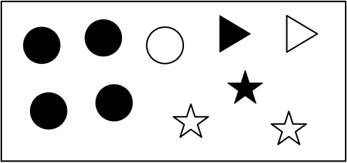
P(\alpha)=\mu(\{\omega\>:\>{\alpha}\mbox{ is true in }{\omega}\}).

Refer to caption — Figure 9.1: Ten possible worlds described by variables $F i l l e d$ and $S h a p e$

Example 9.2.

Consider the ten possible worlds of Figure 9.1, with Boolean variable $F i l l e d$ and with variable $S h a p e$ with domain $\{circle,triangle,star\}$ . Each world is defined by its shape, whether it’s filled, and its position. Suppose the measure of each singleton set of worlds is $0.1$ . Then $P(Shape{\,{=}\,}circle)=0.5$ , as there are five circles and $P(Filled{\,{=}\,}false)=0.4$ , as there are four unfilled shapes. $P(Shape{\,{=}\,}circle\land Filled{\,{=}\,}false)=0.1$ (where “ $\land$ ” means “and”), as there is only one unfilled circle.

If $X$ is a random variable, a probability distribution, $P(X)$ , over $X$ is a function from the domain of $X$ into the real numbers such that, given a value $x\in domain(X)$ , $P(x)$ is the probability of the proposition $X{\,{=}\,}x$ . A probability distribution over a set of variables is a function from the values of those variables into a probability. For example, $P(X,Y)$ is a probability distribution over $X$ and $Y$ such that $P(X{\,{=}\,}x,Y{\,{=}\,}y)$ , where $x\in domain(X)$ and $y\in domain(Y)$ , has the value $P(X{\,{=}\,}x\land Y{\,{=}\,}y)$ , where $X{\,{=}\,}x\land Y{\,{=}\,}y$ is the proposition representing the conjunction (and) of the assignments to the variables, and $P$ is the function on propositions defined above. Whether $P$ refers to a function on propositions or a probability distribution should be clear from the context.

If $X_{1},\dots,X_{n}$ are all of the random variables, an assignment to those random variables corresponds to a world, and the probability of the proposition defining a world is equal to the probability of the world. The distribution over all worlds, $P(X_{1},\dots,X_{n})$ , is called the joint probability distribution.

Beyond Finitely Many Worlds

The definition of probability is straightforward when there are only finitely many worlds. When there are infinitely many worlds, there are some technical issues that need to be confronted.

There are infinitely many worlds when

•

the domain of a variable is infinite, for example, the domain of a variable $h e i g h t$ might be the set of nonnegative real numbers or
•

there are infinitely many variables, for example, there might be a variable for the location of a robot for every millisecond from now infinitely far into the future.

When there are infinitely many worlds there are uncountably many sets of worlds, which is more than can be described with a language with finite sentences. We do not need to define the measure for all sets of worlds, just those that can be defined by logical formulas. This is the basis for the definition of a $\sigma$ -algebra used in many probability texts.

For variables with continuous domains, the probability of $X{\,{=}\,}v$ can be zero for all $v$ , even though the probability of $v_{0}<X<v_{i}$ is positive for $v_{0}<v_{1}$ . For variables with real-valued domains, a probability density function, written as $p$ , is a function from reals into nonnegative reals that integrates to $1$ . The probability that a real-valued variable $X$ has value between $a$ and $b$ is

P(a\leq X\leq b)=\int_{a}^{b}p(X)\hbox{ d}X.

A parametric distribution is one where the probability or density function is described by a formula with free parameters. Not all distributions can be described by formulas, or any finite representation. Sometimes statisticians use the term parametric to mean a distribution described using a fixed, finite number of parameters. A nonparametric distribution is one where the number of parameters is not fixed, such as in a decision tree. (Oddly, nonparametric typically means “many parameters”.)

An alternative is to consider discretization of continuous variables. For example, only consider height to the nearest centimeter or micron, and only consider heights up to some finite number (e.g., a kilometer). Or only consider the location of the robot for a millennium. With finitely many variables, there are only finitely many worlds if the variables are discretized. A challenge is to define representations that work for any (fine enough) discretization.

It is common to work with a parametric distribution when the solutions can be computed analytically and where there is theoretical justification for some particular distribution or the parametric distribution is close enough.

9.1.2 Conditional Probability

Probability is a measure of belief. Beliefs need to be updated when new evidence is observed.

The measure of belief in proposition $h$ given proposition $e$ is called the conditional probability of $h$ given $e$ , written $P(h\mid e)$ .

A proposition $e$ representing the conjunction of all of the agent’s observations of the world is called evidence. Given evidence $e$ , the conditional probability $P(h\mid e)$ is the agent’s posterior probability of $h$ . The probability $P(h)$ is the prior probability of $h$ and is the same as $P(h\mid true)$ because it is the probability before the agent has observed anything.

The evidence used for the posterior probability is everything the agent observes about a particular situation. Everything observed, and not just a few select observations, must be conditioned on to obtain the correct posterior probability.

Example 9.3.

For the diagnostic agent, the prior probability distribution over possible diseases is used before the diagnostic agent finds out about the particular patient. Evidence is obtained through discussions with the patient, observing symptoms, and the results of lab tests. Essentially, any information that the diagnostic agent finds out about the patient is evidence. The agent updates its probability to reflect the new evidence in order to make informed decisions.

Example 9.4.

The information that the delivery robot receives from its sensors is its evidence. When sensors are noisy, the evidence is what is known, such as the particular pattern received by the sensor, not that there is a person in front of the robot. The robot could be mistaken about what is in the world but it knows what information it received.

Semantics of Conditional Probability

Evidence $e$ , where $e$ is a proposition, will rule out all possible worlds that are incompatible with $e$ . Like the definition of logical consequence, the given proposition $e$ selects the possible worlds in which $e$ is true.

Evidence $e$ induces a new measure, $\mu_{e}$ , over sets of worlds. Any set of worlds which all have $e$ false has measure $0$ in $\mu_{e}$ . The measure of a set of worlds for which $e$ is true in all of them is its measure in $\mu$ multiplied by a constant:

\mu_{e}(S)=\left\{\begin{array}[]{ll}c*\mu(S)&\hbox{if }e\mbox{ is true in }% \omega\mbox{ for all }\omega\in S\\ {0}&{\hbox{if }e\mbox{ is false in }\omega\mbox{ for all }\omega\in S}\end{% array}\right.

where $c$ is a constant (that depends on $e$ ) to ensure that $\mu_{e}$ is a proper measure.

For $\mu_{e}$ to be a probability measure over worlds for each $e$ :

	$\displaystyle 1$	$\displaystyle=\mu_{e}(\Omega)$
		$\displaystyle=\mu_{e}(\{w\>:\>e\mbox{ is true in }w\})+\mu_{e}(\{w\>:\>e\mbox{% is false in }w\})$
		$\displaystyle=c*\mu(\{w\>:\>e\mbox{ is true in }w\})+0$
		$\displaystyle=c*P(e).$

Therefore, $c=1/P(e)$ . Thus, the conditional probability is only defined if $P(e)>0$ . This is reasonable, as if $P(e)=0$ , $e$ is impossible.

The conditional probability of proposition $h$ given evidence $e$ is the sum of the conditional probabilities of the possible worlds in which $h$ is true. That is:

	$\displaystyle P(h\mid e)$	$\displaystyle=\mu_{e}(\{\omega\>:\>h\mbox{ is true in }\omega\})$
		$\displaystyle=\mu_{e}(\{\omega\>:\>h\land e\mbox{ is true in }\omega\})+\mu_{e% }(\{\omega\>:\>h\land\neg e\mbox{ is true in }\omega\})$
		$\displaystyle=\frac{1}{P(e)}*\mu(\{\omega\>:\>h\land e\mbox{ is true in }% \omega\})+0$
		$\displaystyle=\frac{P(h\land e)}{P(e)}.$

The last form above is typically given as the definition of conditional probability. Here we have derived it as a consequence of a more basic definition. This more basic definition is used when designing algorithms; set the assignments inconsistent with the observations to have probability zero, and normalize at the end.

Example 9.5.

As in Example 9.2, consider the worlds of Figure 9.1, with each singleton set having a measure of 0.1. Given the evidence $Filled{\,{=}\,}false$ , only four worlds have a nonzero measure, with

P(Shape{\,{=}\,}circle\mid Filled{\,{=}\,}false)=0.25

P(Shape{\,{=}\,}star\mid Filled{\,{=}\,}false)=0.5.

A conditional probability distribution, written $P(X\mid Y)$ where $X$ and $Y$ are variables or sets of variables, is a function of the variables: given a value $x\in domain(X)$ for $X$ and a value $y\in domain(Y)$ for $Y$ , it gives the value $P(X{\,{=}\,}x\mid Y{\,{=}\,}y)$ , where the latter is the conditional probability of the propositions.

The definition of conditional probability allows the decomposition of a conjunction into a product of conditional probabilities. The definition of conditional probability gives $P(e\land h)=P(h\mid e)*P(e)$ . Repeated application of this product can be used to derive the chain rule:

	$\displaystyle P($	$\displaystyle\alpha_{1}\land\alpha_{2}\land\ldots\land\alpha_{n})$
		$\displaystyle=P(\alpha_{n}\mid\alpha_{1}\land\dots\land\alpha_{n-1})*P(\alpha_% {1}\land\dots\land\alpha_{n-1})$
		$\displaystyle=P(\alpha_{n}\mid\alpha_{1}\land\dots\land\alpha_{n-1})\dotsP(% \alpha_{2}\mid\alpha_{1})*P(\alpha_{1})$
		$\displaystyle=\prod_{i=1}^{n}P(\alpha_{i}\mid\alpha_{1}\land\dots\land\alpha_{% i-1})$

where the base case is $P(\alpha_{1}\mid true)=P(\alpha_{1})$ , the empty conjunction being true.

Bayes’ Rule

An agent using probability updates its belief when it observes new evidence. A new piece of evidence is conjoined to the old evidence to form the complete set of evidence. Bayes’ rule specifies how an agent should update its belief in a proposition based on a new piece of evidence.

Suppose an agent has a current belief in proposition $h$ based on evidence $k$ already observed, given by $P(h\mid k)$ , and subsequently observes $e$ . Its new belief in $h$ is $P(h\mid e\land k)$ . Bayes’ rule tells us how to update the agent’s belief in hypothesis $h$ as new evidence arrives.

Proposition 9.1.

(Bayes’ rule) As long as $P(e\mid k)\neq 0$ :

{P(h\mid e\land k)={P(e\mid h\land k)*P(h\mid k)\over P(e\mid k)}}.

This is often written with the background knowledge $k$ implicit. In this case, if $P(e)\neq 0$ , then

{P(h\mid e)={P(e\mid h)*P(h)\over P(e)}}.

$P(e\mid h)$ is the likelihood and $P(h)$ is the prior probability of the hypothesis $h$ . Bayes’ rule states that the posterior probability is proportional to the likelihood times the prior.

Proof.

The commutativity of conjunction means that $h\wedge\mbox{}e$ is equivalent to $e\wedge\mbox{}h$ , and so they have the same probability given $k$ . Using the rule for multiplication in two different ways:

	$\displaystyle P(h\land e\mid k)$	$\displaystyle=P(h\mid e\land k)*P(e\mid k)$
	$\displaystyle\mbox{}=P(e\land h\mid k)$	$\displaystyle=P(e\mid h\land k)*P(h\mid k).$

The theorem follows from dividing the right-hand sides by $P(e\mid k)$ , which is not 0 by assumption. ∎

Generally, one of $P(e\mid h\land k)$ or $P(h\mid e\land k)$ is much easier to estimate than the other. Bayes’ rule is used to compute one from the other.

Example 9.6.

In medical diagnosis, the doctor observes a patient’s symptoms, and would like to know the likely diseases. Thus the doctor would like $P(Disease\mid Symptoms)$ . This is difficult to assess as it depends on the context (e.g., some diseases are more prevalent in hospitals). It is typically easier to assess $P(Symptoms\mid Disease)$ because how the disease gives rise to the symptoms is typically less context dependent. These two are related by Bayes’ rule, where the prior probability of the disease, $P(Disease)$ , reflects the context.

Example 9.7.

The diagnostic assistant may need to know whether the light switch $s_{1}$ of Figure 1.6 is broken or not. You would expect that the electrician who installed the light switch in the past would not know if it is broken now, but would be able to specify how the output of a switch is a function of whether there is power coming into the switch, the switch position, and the status of the switch (whether it is working, shorted, installed upside-down, etc.). The prior probability for the switch being broken depends on the maker of the switch and how old it is. Bayes’ rule lets an agent infer the status of the switch given the prior and the evidence.

9.1.3 Expected Values

The expected value of a numerical random variable (one whose domain is the real numbers or a subset of the reals) is the variable’s weighted average value, where sets of worlds with higher probability have higher weight.

Let $X$ be a numerical random variable. The expected value of $X$ , written ${{\mathcal{E}}_{P}(X)}$ , with respect to probability $P$ is

\displaystyle{\mathcal{E}}_{P}(X)

\displaystyle=\sum_{v\in domain(X)}v*P(X{\,{=}\,}v)

when the domain is $X$ is finite or countable. When the domain is continuous, the sum becomes an integral.

One special case is if $\alpha$ is a proposition, treating $t r u e$ as 1 and $f a l s e$ as 0, where ${\mathcal{E}}_{P}(\alpha)=P(\alpha)$ .

Example 9.8.

In an electrical domain, if $number\_of\_broken\_switches$ is the number of switches broken:

{{\mathcal{E}}_{P}(number\_of\_broken\_switches)}

would give the expected number of broken switches given by probability distribution $P$ . If the world acted according to the probability distribution $P$ , this would give the long-run average number of broken switches. If there were three switches, each with a probability of $0.7$ of being broken independently of the others, the expected number of broken switches is

\displaystyle 0*0.3^{3}+1*3*0.7*0.3^{2}+2*3*0.7^{2}*0.3+3*0.7^{3}=2.01

where $0.3^{3}$ is the probability that no switches are broken, $0.7*0.3^{2}$ is the probability that one switch is broken, which is multiplied by 3 as there are three ways that one switch can be broken.

In a manner analogous to the semantic definition of conditional probability, the conditional expected value of $X$ conditioned on evidence $e$ , written ${\mathcal{E}}(X\mid e)$ , is

\displaystyle{\mathcal{E}}(X\mid e)

\displaystyle=\sum_{v\in domain(X)}v*P(X{\,{=}\,}v\mid e).

Example 9.9.

The expected number of broken switches given that light $l_{1}$ is not lit is given by

{\mathcal{E}}(number\_of\_broken\_switches\mid\neg lit(l_{1})).

This is obtained by averaging the number of broken switches over all of the worlds in which light $l_{1}$ is not lit.

If a variable is Boolean, with true represented as 1 and false as 0, the expected value is the probability of the variable. Thus any algorithms for expected values can also be used to compute probabilities, and any theorems about expected values are also directly applicable to probabilities.

Artificial Intelligence 3E