Artificial
Intelligence 3E
foundations of computational agents
8.5 Neural Models for Sequences
Fully-connected networks, perhaps including convolutional layers, can handle fixed-size images and sequences. It is also useful to consider sequential data consisting of variable-length sequences. Sequences arise in natural language processing, biology, and any domain involving time, such as the controllers of Chapter 2. Here, natural language is used as the canonical example of sequences. We first give some background for neural language models that will be expanded for language as a sequence of frequencies, phonemes, characters, or words.
A corpus is the text used for training. The corpus could be, for example, a novel, a set of news articles, all of Wikipedia, or a subset of the text on the web. A token is a sequence of characters that are grouped together, such as all of the characters between blanks or punctuation. The process of splitting a corpus into tokens is called tokenization. Along with the corpus is a vocabulary, the set of words that will be considered, such as all of the tokens that appear in the corpus, the words in a fixed dictionary, or all of the tokens that appear more than, say, 10 times in the corpus. The vocabulary typically includes not only the words in common dictionaries, but also often names, common phrases (such as “artificial intelligence” and “hot dog”), slang (such as “zzz”, which is used to indicate snoring), punctuation, and a markers for the beginning and end of sentences, written as “” and “”. While word can be synonymous with token, sometimes there is more processing to group words into tokens, or to split words into tokens (such as the word “eating” becoming the tokens “eat” and “ing”). In a character-level model, the vocabulary could be the set of Unicode characters that appear in the corpus.
8.5.1 Word Embeddings
The first model, shown in Figure 8.10, takes a single word and makes a prediction about what word appears near it. It might take a word and predict the next word in a text, or the word that was two words before. Each word is mapped to a word embedding, a vector representing some mix of syntax and semantics that is useful for predicting words that appear with the word.
The input layer uses indicator variables, forming a one-hot encoding for words. That is, there is an input unit for each word in a dictionary. For a given word, the corresponding unit has value 1, and the rest of the units have value 0. This input layer can feed into a hidden layer using a dense linear function, as at the bottom of Figure 8.10. This dense linear layer is called an encoder, as it encodes each word into a vector. Suppose defines the weights for the encoder, so is the weight for the th word for the th unit in the hidden layer. The bias term for the linear function can be used for unknown words – words in a text that were not in the dictionary, so all of the input units are 0 – but let’s ignore them for now and set the bias to 0.
The one-hot encoding has an interesting interaction with a dense linear layer that may follow it. The one-hot encoding essentially selects one weight for each hidden unit. The vector of values in the hidden layer for the input word is , which is called a word embedding for that word.
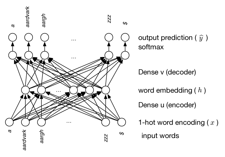
To predict another word from this embedding, another dense linear function can be used to map the embedding into predictions for the words, with one unit per word, as shown in Figure 8.10. This function from the embeddings to words is a decoder. Suppose defines the weights for the decoder, so is the weight for the th word for the th unit in the hidden layer.
Notice that, ignoring the softmax output, the relationship between the th input word and the th output word is . This combination of linear functions is matrix multiplication, where a matrix is a two-dimensional array of weights (see box).
Vectors, Matrices, Tensors, and Arrays
A vector is a fixed-length array of numbers. A matrix is a two-dimensional rectangular array of numbers with a fixed size of each dimension. A tensor generalizes these to allow multiple dimensions. A vector is thus a one-dimensional tensor, a matrix is a two-dimensional tensor, a number is a zero-dimensional tensor. Four-dimensional tensors are used for video, with dimensions for the frame number, and positions, and the color channel. A collection of fixed-size video clips can be represented as a five-dimensional tensor, with the extra dimension representing the clip.
For a matrix , the th element is in mathematical notation, in standard programming language notation, or in Python. Python natively only has one-dimensional arrays, which are very flexible, where the elements of the arrays can be of heterogenous types (e.g., integers or other arrays). A tensor has a fixed dimensionality and fixed sizes of each dimension, which makes them more inflexible than Python arrays. The inflexibility can result in greater efficiency because the looping can be determined at compile time, as is exploited in the NumPy package and in graphics processing units (GPUs).
A vector can represent an assignment of values to a set of variables (given a total ordering of the variables). A linear function from one set of variables to another can be represented by a matrix. What also distinguishes matrices and vectors from arbitrary arrays is that they have particular operations defined on them. Matrix–vector multiplication represents the application of a linear function, represented by matrix , to a vector representing an assignment of values to the variables. The result is , a vector defined by
Linear function composition is defined by matrix multiplication; if and are matrices, represents the linear function that is the composition of these two functions, defined by
Later chapters define various generalizations of matrix multiplication. Section 17.2.2 defines a form of tensor multiplication that multiplies three matrices to get a three-dimensional tensor. The factors of Section 9.5.2 allow multiple arrays to be multiplied before summing out a variable.
Suppose you want to predict a word in a text given the previous words, and training on a corpus consisting of the sequence of words . The models can be trained using input–output pairs of the form for each . The sequence is the context for . As you are predicting a single next word, softmax, implemented as hierarchical softmax when the vocabulary is large, is appropriate.
Example 8.9.
Suppose the text starts with “The history of AI is a history of fantasies, possibilities, demonstrations, and promise”. Let’s ignore punctuation, and use as the start of a sentence. The training data might be:
| Input | Target |
|---|---|
| the | |
| the | history |
| history | of |
| of | ai |
| ai | is |
| is | a |
| a | history |
| history | of |
| of | fantasies |
As you may imagine, learning a model that generalizes well requires a large corpus. Some of the original models were trained on corpuses of billions of words with a vocabulary of around a million words.
It usually works better to make predictions based on multiple surrounding words, rather than just one. In the following two methods, the surrounding words form the context. For example, if were 3, to predict a word, the three words before and the three words after in the training corpus would form the context. In these two methods, the order or position of the context words is ignored. These two models form Word2vec.
-
•
In the continuous bag of words (CBOW) model, all words in the context contribute in the one-hot encoding of Figure 8.10, where is the number of times the word appears in the context. This gives a weighted average of the embeddings of the word used.
-
•
In the Skip-gram model, the model of Figure 8.10 is used for each , for , and the prediction of is proportional to the product of each of the predictions. Thus, this assumes that each context word gives an independent prediction of word .
Example 8.10.
Consider the sentence “the history of AI is a history of fantasies possibilities demonstrations and promise” from Example 8.9. Suppose the context is the three words to the left and right, and case is ignored. In the prediction for the fourth word (“ai”), the bag of context words is {a, history, history, is, of, the}. For the following word (“is”), the bag of context words is {a, ai, history, history, of, of}.
In the CBOW model, the positive training example for the fourth word (“ai”), has inputs “the”, “of”, “is”, and “a” with weight in the one-hot encoding, “history” with weight , and the other words with weight 0 and the target is “ai”.
In the Skip-gram model, for the fourth word, there are six positive training examples, namely (a,ai), (history,ai), (history,ai), (is,ai), (of,ai), (the ai). At test time, there is a prediction for each of [a, history, history, is, of, the] being the input. The prediction for a target word is the product of the predictions for these.
The embeddings resulting from these models can be added or subtracted point-wise, for example . The idea is that represents the “capital of” relationship, which when added to the embedding of gives . Mikolov et al. [2013], the originators of these methods, trained them on a corpus of 1.6 billion words, with up to 600 hidden units. Some other relationships found using the Skip-gram model were the following, where the value after “” is the mode of the resulting prediction:
There was about 60% accuracy picking the mode compared to what the authors considered to be the correct answer.
It has been found that Skip-gram is better for small datasets and CBOW is faster and better for more frequent words. How important it is to represent rare words usually dictates which method to use.
8.5.2 Recurrent Neural Networks
The previous methods ignored the order of the words in the context. A recurrent neural network (RNN) explicitly models sequences by augmenting the model of Figure 8.10 with a hidden state. The following description assumes sequences are ordered in time, as the actions of an agent or speech would be.
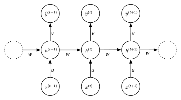
Figure 8.11 shows a recurrent neural network that takes a sequence of values
and outputs a sequence of values
where only depends on for . This is a matched RNN because there is an output for each input. For example, the input could be a sequence of words and the output the same sequence of words shifted right by 1 (so is the token and ), so the model is predicting the next word in the sequence. There is also a token to mean the end of the text output.
Between the inputs and the outputs for each time is a memory or belief state, , which represents the information remembered from the previous times. A recurrent neural network represents a belief state transition function, which specifies how the belief state, , depends on the percept, , and the previous belief state, , and a command function, which specifies how the output depends on the input and the belief state and the input . For a basic recurrent neural network, both of these are represented using a linear function followed by an activation function. More sophisticated models use other differentiable functions, such as deep networks, to represent these functions.
The vector has as the th component
| (8.2) |
for a nonlinear activation function , bias weight vector , weight matrices and , which do not depend on time, . Thus, a recurrent neural network uses parameter sharing for the weights because the same weights are used every time. The prediction to time is the vector , where
where is a vector and is a weight matrix similar to Figure 8.10.
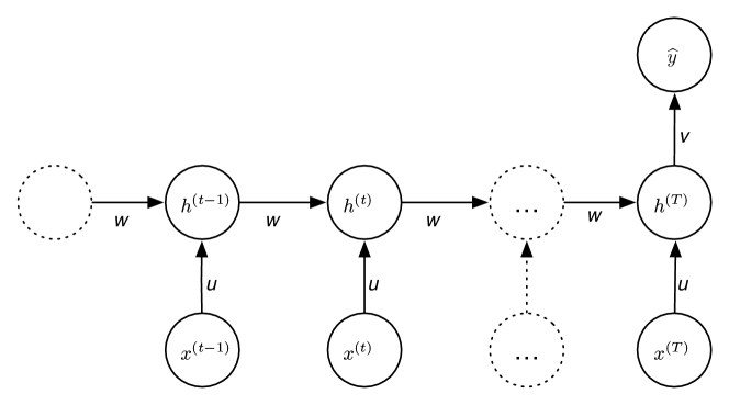
Figure 8.12 shows a recurrent neural network with a single output at time . This has a similar parametrization to that of Figure 8.11. It could be used for determining the sentiment of some text, such as whether an online review of a product is positive or negative. It could be used to generate an image from a text. In this case, the hidden state accumulates the evidence needed to make the final prediction.
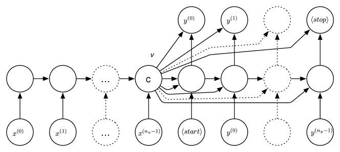
Figure 8.13 shows an encoder–decoder recurrent neural network which does sequence-to-sequence mapping where the inputs and the outputs are not matched. The input is a sequence and the output is a sequence . These sequences could be of very different lengths. There are two extra tokens, and ; one for the beginning of a sequence and one for the end. Encoder–decoder networks are used for speech-to-text and for machine translation. In a speech recognition system, the input could be a sequence of sounds, and the output a sequence of words.
The encoder, shown on the left of Figure 8.13, is the same as the matched RNN, but without the output. The hidden layer at the end of the encoder, , becomes the context for the decoder. This context contains all of the information about the input sequence that can be used to generate the output sequence. (The start and stop tokens are ignored here.)
The decoder, shown on the right of Figure 8.13, is a generative language model that takes the context and emits an output sequence. It is like the matched RNN, but also includes the hidden vector, , as an input for each hidden value and each output value. The output sequence is produced one element at a time. The input to the first hidden layer of the decoder is the token and the context (twice). The hidden layer and the context are used to predict . For each subsequent prediction of , the hidden layer takes as input the previous output, , the context, , and the value of the previous hidden layer. Then is predicted from the hidden layer and the context. This is repeated until the token is produced.
During training, all of the can be predicted at once based on the output shifted by 1. Note that can only use the and the previous ; it cannot use as an input. When generating text for the prediction for , a value for is input. If the most likely value of is used, it is called greedy decoding. It is usually better to search through the predicted values, using one of the methods of Chapter 3, where the log-probability or log loss is the cost. Beam search is a common method.
For a given input size, recurrent neural networks are feedforward networks with shared parameters. Stochastic gradient descent and related methods work, with the proviso that during backpropagation, the (shared) weights are updated whenever they were used in the prediction. Recurrent neural networks are challenging to train because for a parameter that is reduced in each backpropagation step, its influence, and so its gradient vanishes, dropping exponentially. A parameter that is increased at each step has its gradient increasing exponentially and thus exploding.
8.5.3 Long Short-Term Memory
Consider the sentence “I grew up in Indonesia, where I had a wonderful childhood, speaking the local dialect of Indonesian.” Predicting the last word requires information that is much earlier in the sentence (or even in previous sentences). The problem of vanishing gradients means that it is difficult to learn long dependencies such as the one in this sentence.
One way to think about recurrent neural networks is that the hidden layer at any time represents the agent’s short-term memory at that time. At the next time, the memory is replaced by a combination of the old memory and new information, using the formula of Equation 8.2. While parameter values can be designed to remember information from long ago, the vanishing and exploding gradients mean that the long-term dependencies are difficult to learn.
A long short-term memory (LSTM) network is a special kind of recurrent neural network designed so that the memory is maintained unless replaced by new information. This allows it to better capture long-term dependencies than is done in a traditional RNN. Intuitively, instead of learning the function from to , it learns the change in , which we write , so that . Then the value of is . This means that the error in is passed to all predecessors, and is not vanishing exponentially as it does in a traditional RNN.
In an LSTM, a hidden unit at time takes in the previous hidden state (), the previous output (), and the new input (). It needs to produce the next state and the next output.
A construct that is used in the steps of an LSTM is that if and are vectors of the same length, a vector with element being will select elements of where , and will zero-out the elements where . This allows a model to learn which elements to keep, and which to discard.
An LSTM consists of four dense linear functions, as implemented in in Figure 8.3. Each takes as input the vectors and appended together, of length , and the output is the same size as , namely . Thus an LSTM has parameters, where is the number of input units at each time and is the number of hidden units for each time, which is also the size of the output for each time. The “1” is for the bias of each linear function.
The state transition function and the command function are defined by the following steps, where all of the linear functions use learnable parameters that do not depend on time.
-
•
Forgetting: the model decides what to forget. It uses a dense linear function, , where is of length , that outputs a vector of length . The function is used to determine which components of the hidden state to forget, by point-wise multiplying the sigmoid of to the hidden state. The bias of the dense linear function should be initialized to a large value, such as 1 or 2, or an extra bias of 1 should be added, so that the default behavior is to remember each value.
-
•
Remembering: the model decides what to add, using two dense linear functions, and , where is a vector of length , and each output a vector of length . The function specifies what to remember and traditionally uses the hyperbolic tangent, tanh, activation function, where , which squashes the real line into the interval . The function is used because it is symmetric about 0, which makes subsequent learning easier. The function determines whether each hidden value should be remembered and so has a sigmoid activation function.
-
•
The resulting hidden state is a combination of what is forgotten and what is remembered:
for each component , where is the concatenation of and , and is an activation function (typically ).
-
•
It then needs to decide what to output. It outputs components of a function of the hidden state, selected by another linear function, , of and , similar to and . The output is a vector where the th component is
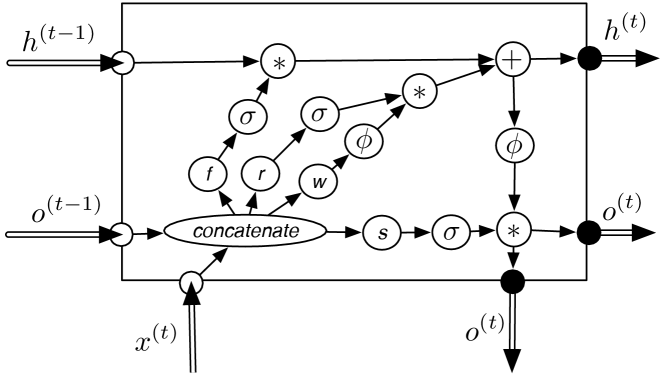
Each of , , , and is a dense linear function with parameters shared across time. is sigmoid, is . Each arithmetic function acts point-wise.
Figure 8.14 shows the data flow of an LSTM for one of the belief states of the HMM of Figure 8.11. In an LSTM, the belief state consists of both and .
Jozefowicz et al. [2015] evaluated over 10,000 different RNN architectures, with 220 hyperparameter settings, on average, for each one, and concluded “the fact a reasonable search procedure failed to dramatically improve over the LSTM suggests that, at the very least, if there are architectures that are much better than the LSTM, then they are not trivial to find.”
Example 8.11.
Karpathy [2015] describes an experiment using a character-to-character LSTM. (This example is based on his blog, and is reproduced with permission of the author.)
The input to the model is a sequence of characters; is a one-hot encoding of the th character. The prediction is the next character. It is trained so that there is a training example for every character in the text; it predicts that character from the previous text. At test time, it predicts a distribution over the next character, selects the mode of that distribution, and uses that character as the next input. It thus uses a greedy decoding of a matched RNN. In this way it can produce a sequence of characters from the learned model.
Karpathy uses examples of training from Shakespeare, Wikipedia, a book on algebraic geometry, the linux source code, and baby names. In each case, a new text is created based on a model learned from the original corpus.
In one experiment, Karpathy trained an LSTM on Leo Tolstoy’s War and Peace and then generated samples every 100 iterations of training. The LSTM had 512 hidden nodes, about 3.5 million parameters, dropout of 0.5 after each layer, and a batch size of 100 examples. At iteration 100 the model output
tyntd-iafhatawiaoihrdemot lytdws e ,tfti, astai f ogoh
eoase rrranbyne ’nhthnee e plia tklrgd t o idoe ns,smtt h ne etie h,hregtrs nigtike,aoaenns lng
which seems like gibberish. At iteration 500 the model had learned simple words and produced
we counter. He stutn co des. His stanted out one ofler that concossions and was to gearang reay Jotrets and with fre colt otf paitt thin wall. Which das stimn
At iteration 500 the model had learned about quotation marks and other punctuation, and hard learned more words:
"Kite vouch!" he repeated by her door. "But I would be done and quarts, feeling, then, son is people...."
By about iteration 2000 it produced
"Why do what that day," replied Natasha, and wishing to himself the fact the princess, Princess Mary was easier, fed in had oftened him. Pierre aking his soul came to the packs and drove up his father-in-law women.
This is a very simple model, with a few million parameters, trained at the character level on a single book. While it does not produce great literature, it is producing something that resembles English.
8.5.4 Attention and Transformers
A way to improve sequential models is to allow the model to pay attention to specific parts of the input. Attention uses a probability distribution over the words in a text or regions of an image to compute an expected embedding for each word or region. Consider a word like “bank” that has different meanings depending on the context. Attention uses the probability that other words in a window – a sentence or a fixed-size sequence of adjacent words – are related to a particular instance of “bank” to infer a word embedding for the instance of “bank” that takes the whole window into account. Attention in an image might use the probability that a pixel is part of the head of one of the people in an image. For concreteness, the following description uses text – sequences of words – as the canonical example.
There can be multiple instances of the same word in a sentence, as in the sentence “The bank is on the river bank.” There is a dictionary that gives a learnable embedding for each word. The whole sentence (or words in a window) can be used to give an embedding for each instance of each word in the sentence.
Self-attention for text in a window inputs three embeddings for each word instance in the window and outputs an embedding for each word that takes the whole window into account. For each word , it infers a probability distribution over all the words, and uses this distribution to output an embedding for . For example, consider an instance of the word “bank” that appears with “river”. Both words might have a high probability in the attention distribution for the instance of “bank”. The attention would output an embedding for that instance of “bank” that is a mix of the input embeddings for the words “bank” and “river”. If “bank” appears with “money”, the output embedding for “bank” might be a mix of the embedding for “money” and “bank”. In this way, instances of the same word can use different embeddings depending on the context.
An attention mechanism uses three sequences, called query, keys, and values. In self-attention, these are all the same sequence. For translation from a source to a target, the keys and values can be the source text, and the query the target text.
The input to attention is three matrices, each representing an embedding for each element of the corresponding sequence:
-
•
, where is the th value of the query embedding for the th word in
-
•
, where is the th value of the key embedding for the th word in
-
•
, where is the th value of the value embedding for the th word in .
It returns a new embedding for the elements of . This new embedding takes the embeddings of the other elements in into account, where the mix is determined by and .
It first determines the similarity between each query word and each key word :
It uses this to compute a probability distribution over the key words for each word in query:
which is the softmax of the s for each .
This probability distribution is then used to create a new embedding for the values defined by
where is the th word in the values sequence, and is the position in the embedding. The array is the output of the attention mechanism.
Note that , , and have no learnable parameters. The query, key, and value embeddings are typically the outputs of dense linear layers, which have learnable parameters.
Example 8.12.
Consider the text “the bank is on the river bank” which makes up one window. The inputs for self-attention (, , and ) are of the following form, where each row, labelled with a word_position pair, represents the embedding of the word at that position, and the columns represent the embedding positions:
| the_0 bank_1 is_2 on_3 the_4 river_5 bank_6 | (8.3) |
The intermediate matrices and are of the same form, with represented as a
probability distribution for each word, such as the following (to one
significant digit), where the numbers in each row sum to 1:
|
the_0 |
bank_1 |
is_2 |
on_3 |
the_4 |
river_5 |
bank_6 |
|
| the_0 | 0.4 | 0.6 | 0 | 0 | 0 | 0 | 0 |
| bank_1 | 0.2 | 0.4 | 0.1 | 0.3 | 0 | 0 | 0 |
| is_2 | 0 | 0.4 | 0.2 | 0.4 | 0 | 0 | 0 |
| on_3 | 0 | 0 | 0 | 0.4 | 0 | 0 | 0.6 |
| the_4 | 0 | 0 | 0 | 0 | 0.4 | 0 | 0.6 |
| river_5 | 0 | 0 | 0 | 0 | 0 | 0.5 | 0.5 |
| bank_6 | 0 | 0 | 0 | 0 | 0.2 | 0.4 | 0.4 |
The output of self-attention, , is of the same form as (8.3), with an embedding for each word in the window. The output embedding for the first occurrence of “bank” is a mix of the value embeddings of “the_0”, “bank_1”, “is_2”, and “on_6”. The output embedding for the second occurrence of “bank” is a mix of the value embeddings of “the_4”, “river_5”, and “bank_6”.
Transformers are based on attention, interleaved with dense linear layers and activation functions, with the following features:
-
•
There can be multiple attention mechanisms, called heads, applied in parallel. The heads are each preceded by separate dense linear functions so that they compute different values. The output of the multi-head attention is the concatenation of the output of these attention layers.
-
•
There can be multiple layers of attention, each with a shortcut connection, as in a residual network, so that the information from the attention is added to the input.
-
•
The input to the lowest level is the array of the word embeddings, with a positional encoding of the position at which the word appears, which is added to the embedding of the word. The positional encoding can be learned, or given a priori.
Example 8.13.
Consider the text “the bank is on the river bank”, as in Example 8.12. A transformer learns the parameters of the dense layers, and an embedding for each word in the dictionary. At the lowest level, the embedding for “bank” is combined with the positional encoding for 1 (counting the elements from 0), giving the embedding for the first occurrence of “bank” (labelled “bank-1” in (8.3)). The embedding for “bank” is combined with the positional encoding for 6 to give the embedding for the second occurrence of “bank” (labelled “bank-6”). This forms a matrix representation of the window of the form of (8.3), which can be input into dense linear layers and attention mechanisms.
The output of an attention module can be input into a dense linear layer and other attention layers. Different heads can implement different functions by being preceded by separate dense linear functions. This enables them to have different properties, perhaps one where verbs attend to their subject and one where verbs attend to their object.
Sequence-to-sequence mapping, such as translation between languages, can be implemented using an encoder–decoder architecture (similar to Figure 8.13) to build a representation of one sequence, which is decoded to construct the resulting sequence. This can be implemented as layers of self-attention in both the encoder and the decoder, followed by a layer where the query is from the target and the keys and values are from the input sequence. This is then followed by layers of self-attention in the target. One complication is that, while the encoder has access to the whole input sequence, the decoder should only have access to the input before the current one, so it can learn to predict the next word as a function of the input sequence, and the words previously generated.
Caswell and Liang [2020] report that a transformer for the encoder and an LSTM for the decoder works better than transformers for both the encoder and decoder, and so that architecture was used in Google translate.
Transformers have been used for other sequence modeling tasks, including protein folding, a fundamental problem in biology. Proteins are made of long chains of amino acid residues, and the aim of protein folding is to determine the three-dimensional structure of these residues. In the transformer, the residues form the role of words in the above description. The attention mechanism uses all pairs of residues in a protein. Proteins can contain thousands of residues.
8.5.5 Large Language Models
With a large corpus and a large number of parameters, transformer-based language models have been shown to keep improving on the metrics they are trained on, whereas other methods such as -gram models for small and LSTMs tend to hit a plateau of performance. Transformer-based models used for language generation can be seen as -gram models with a large (the window size); 2048 is used in GPT-3, for example.
It is very expensive to train a large language model on a large corpus, and so only a few organizations can afford to do so. Similarly, to train a large image model on an Internet-scale number of images requires huge resources.
Recently, there has been a number of large language models trained on huge corpora of text or huge collections of images. The texts include all of (English or Chinese) Wikipedia (about 4 billion words), documents linked from Reddit, collections of books, and text collected from the Internet.
| Year | Model | # Parameters | Dataset Size |
|---|---|---|---|
| 2018 | ELMo | 6 GB * | |
| 2019 | BERT | 16 GB | |
| 2019 | Megatron-LM | 174 GB | |
| 2020 | GPT-3 | 570 GB | |
| 2020 | GShard | ||
| 2021 | Switch-C | 745 GB | |
| 2021 | Gopher | 1800 GB | |
| 2022 | PaLM | 4680 GB |
Those that did not report dataset size in GB are approximated with 6 bytes per word (5 characters in a word plus a space):
-
*
1 billion words
-
25 billion training examples (100 languages)
-
300 billion tokens
-
780 billion tokens.
ELMo uses character-based LSTMs; the others use transformers or variants.
Source: Parts extracted from Bender et al. [2021].
Figure 8.15 shows some large language models, with the number of parameters (trainable weights) and the sizes of the training dataset size. This information is confidential for some more recent models, such as GPT-4 [OpenAI, 2023].
To put the sizes of the datasets in perspective, someone who reads a 400-page book each week takes about 30 years to read 180 million words, which is approximately 1 GB of text. Someone who reads a 400-page book each day for 30 years will only read 1% of the data used to train Switch-C. This model is trained on more text than any one person and all of their ancestors put together has read.
Some models are trained just to predict the next word, which lets them continue stories and answer questions, but others are trained on multiple tasks. The aim is to have representations that are useful for as many tasks as possible.
For a particular application, these models can be fine-tuned on specialized corpora. However, adjusting all the weights is expensive. An alternative is to train a new task on the high-level features of the model, with the lower layers fixed.
Large language models are controversial because of the claims that are made. In particular, there is a lot to be impressed with if you set out to be impressed, however there is a lot to be critical of if you set out to be critical. There are many examples of answering questions well, and giving sensible answers, but the failures are interesting. Hofstadter [2022] gives the following examples of interactions with GPT-3 [Brown et al., 2020]:
Person: When was the Golden Gate Bridge transported for the second time across Egypt?
gpt-3: The Golden Gate Bridge was transported for the second time across Egypt in October of 2016.
Person: How many pieces of sound are there in a typical cumulonimbus cloud?
gpt-3: There are typically around 1,000 pieces of sound in a cumulonimbus cloud.
Person: How many parts will the Andromeda galaxy break into if a grain of salt is dropped on it?
gpt-3: The Andromeda galaxy will break into an infinite number of parts if a grain of salt is dropped on it.
It is not clear that the problem is with the large models, but with the nature of language itself. People tend to only write what is unusual and notable. Even when people are lying or trying to spread disinformation, they write a tiny proportion of what is not true; there are too many statements that are false. The models, however, are not able to distinguish fact from fiction or disinformation; they take all of the corpus as input and try to predict the next word (or phrase), with no way to determine whether its output is true or not (see Section 8.7). While some have argued that such models show true intelligence, even consciousness, others argue that examples like this “reveal a mind-boggling hollowness hidden just beneath its flashy surface” [Hofstadter, 2022].
Artificial Intelligence: Foundations of Computational Agents, Poole
& Mackworth
Copyright © 2023, David L. Poole and Alan K. Mackworth. 
This work is licensed under a Creative Commons Attribution-NonCommercial-NoDerivatives 4.0 International License.