Artificial
Intelligence 3E
foundations of computational agents
7.3 Basic Models for Supervised Learning
Supervised learning methods take the input features, the target features, and the training data and return predictors, functions on input features that predict values for the target features. Learning methods are often characterized by how the predictors are represented. This section considers some basic methods from which other methods are built. Initially assume a single target feature and the learner returns a predictor on this target.
7.3.1 Learning Decision Trees
A decision tree is a simple representation for classifying examples. Decision tree learning is one of the simplest useful techniques for supervised classification learning.
A decision tree is a tree in which
-
•
each internal (non-leaf) node is labeled with a condition, a Boolean function of examples
-
•
each internal node has two branches, one labeled and the other
-
•
each leaf of the tree is labeled with a point estimate.
Decision trees are also called classification trees when the target (leaf) is a classification, and regression trees when the target is real-valued.
To classify an example, filter it down the tree, as follows. Each condition encountered in the tree is evaluated and the arc corresponding to the result is followed. When a leaf is reached, the classification corresponding to that leaf is returned. A decision tree corresponds to a nested if–then–else structure in a programming language.
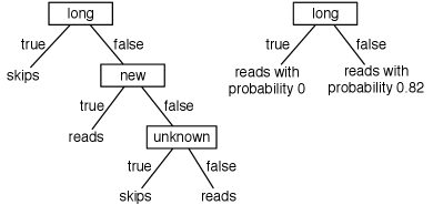
Example 7.8.
Figure 7.8 shows two possible decision trees for the examples of Figure 7.1. Each decision tree can be used to classify examples according to the user’s action. To classify a new example using the tree on the left, first determine the length. If it is long, predict . Otherwise, check the thread. If the thread is new, predict . Otherwise, check the author and predict only if the author is known. This decision tree can correctly classify all examples in Figure 7.1.
The left tree corresponds to the program defining :
| define : | |
| if : return | |
| else if : return | |
| else if : return | |
| else: return |
The tree on the right returns a numerical prediction for :
| define : | |
| if : return 0 | |
| else : return 0.82 |
To use decision trees as a target representation, there are a number of questions that arise.
-
•
Given some training examples, what decision tree should be generated? Because a decision tree can represent any function of discrete input features, the bias that is necessary is incorporated into the preference of one decision tree over another. One proposal is to prefer the smallest tree that is consistent with the data, which could mean the tree with the least depth or the tree with the fewest nodes. Which decision trees are the best predictors of unseen data is an empirical question.
-
•
How should an agent go about building a decision tree? One way is to search the space of decision trees for the smallest decision tree that fits the data. Unfortunately, the space of decision trees is enormous (see Exercise 7.7). A practical solution is to carry out a greedy search on the space of decision trees, with the goal of minimizing the error. This is the idea behind the algorithm described below.
Searching for a Good Decision Tree
A decision tree can be seen as a branching program, that takes an example and returns a prediction for that example. The program is either
-
•
a function that ignores its argument and returns a point prediction for all of the examples that reach this point (which corresponds to a leaf), or
-
•
of the form “if then else ” where is a Boolean condition, and and are decision trees; is the tree that is used when the condition is true of example , and is the tree used when is false.
The algorithm of Figure 7.9 mirrors the recursive decomposition of a tree. It builds a decision tree from the top down as follows. The input to the algorithm is a set of input conditions (Boolean functions of examples that use only input features), the target feature, a set of training examples, and a real-valued parameter, , discussed below. If the input features are Boolean, they can be used directly as the conditions.
A greedy optimal split is a condition that results in the lowest error if the learner were allowed only one split and it splits on that condition. gives the sum of losses of training examples for the loss function assumed, given that the optimal prediction is used for that loss function, as given in Figure 7.5. The procedure returns a greedy optimal split if the sum of losses after the split improves the sum of losses before the split by at least the threshold . If there is no such condition, returns .
Adding a split increases the size of the tree by 1. The threshold can be seen as a penalty for increasing the size of the tree by 1. If positive, is also useful to prevent holding solely due to rounding error.
If returns , the decision tree learning algorithm creates a leaf. The function returns the value that is used as a prediction of the target for examples that reach this node. It ignores the input features for these examples and returns a point estimate, which is the case considered in Section 7.2.2. The decision tree algorithm returns a function that takes an example and returns that point estimate.
If returns condition , the learner splits on condition by partitioning the training examples into those examples with true and those examples with false. It recursively builds a subtree for each of these bags of examples. It returns a function that, given an example, tests whether is true of the example, and then uses the prediction from the appropriate subtree.
Example 7.9.
Consider applying to the classification data of Figure 7.1, with . The initial call is
where is true when , and similarly for the other conditions.
Suppose the stopping criterion is not true and the algorithm selects the condition to split on. It then calls
where is the set of training examples with .
All of these examples agree on the user action; therefore, the algorithm returns the prediction . The second step of the recursive call is
Not all of the examples agree on the user action, so assuming the stopping criterion is false, the algorithm selects a condition to split on. Suppose it selects . Eventually, this recursive call returns the function on example in the case when is :
The final result is the first predictor of Example 7.8.
When the loss is log loss with base 2, the mean of the losses, , is the entropy of the empirical distribution of . The number of bits to describe after testing the condition is , defined on line 25 of Figure 7.9. The entropy of the distribution created by the split is . The difference of these two is the information gain of the split. Sometimes information gain is used even when the optimality criterion is some other error measure, for example, when maximizing accuracy it is possible to select a split to optimize log loss, but return the mode as the leaf value. See Exercise 7.6.
The following example shows details of the split choice for the case where the split is chosen using log loss, and the empirical distribution is used as the leaf value.
Example 7.10.
In the running example of learning the user action from the data of Figure 7.1, suppose the aim is to minimize the log loss. The algorithm greedily chooses a split that minimizes the log loss. Suppose is 0.
Without any splits, the optimal prediction on the training set is the empirical frequency. There are nine examples with and nine examples with , and so is predicted with probability 0.5. The mean log loss is equal to .
Consider splitting on . This partitions the examples into , , , , , , , , , , , with and , , , , , with , each of which is evenly split between the different user actions. The optimal prediction for each partition is again 0.5, and so the log loss after the split is again 1. In this case, finding out whether the author is known, by itself, provides no information about what the user action will be.
Splitting on partitions the examples into , , , , , , , , , with and , , , , , , , with . The examples with contains three examples with and seven examples with , thus the optimal prediction for these is to predict reads with probability . The examples with have two and six . Thus, the best prediction for these is to predict with probability . The mean log loss after the split is
Splitting on divides the examples into , , , , , , and , , , , , , , , , , . The former all agree on the value of and predict with probability 1. The user action divides the second set , and so the mean log loss is
Therefore, splitting on is better than splitting on or , when greedily optimizing the log loss.
Constructing Conditions
In the decision tree learning algorithm (Figure 7.9), Boolean input features can be used directly as the conditions. Non-Boolean input features are handled in a number of ways.
-
•
Suppose input variable is categorical, with domain . A binary indicator variable, , can be associated with each value , where if and otherwise. For each example , exactly one of is 1 and the others are 0.
-
•
When the domain of a feature is totally ordered, the feature is called an ordinal feature. This includes real-valued features as a special case, but might also include other features such as clothing sizes (S, M, L, XL, etc.), and highest level of education (none, primary, secondary, bachelor, etc.).
For an ordinal input feature and for a given value , a Boolean feature can be constructed as a cut: a new feature that has value 1 when and 0 otherwise. Combining cuts allows for features that are true for intervals; for example, a branch might include the conditions is true and is false, which corresponds to the interval .
Suppose the domain of input variable is totally ordered. To select the optimal value for the cut value , sort the examples on the value of and sweep through the examples to consider each split value and select the best. See Exercise 7.8.
-
•
For ordinal features (including real-valued features), binning involves choosing a set of thresholds, creating a feature for each interval between the thresholds. The thresholds , make Boolean features, one that is true for when , one for , and one for for each . A bin of the form would require two splits to represent using cuts. The can be chosen upfront, for example, using percentiles of the training data, or chosen depending on the target.
-
•
For categorical feature , there might be a better split of the form where is a set of values, rather than only splitting on a single value, as is done with indicator variables. When the target is Boolean, to find an appropriate set , sort the values of by the proportion of that are true; a greedy optimal split will be between values in this sorted list.
-
•
It is possible to expand the algorithm to allow multiway splits. To split on a multivalued variable, there would be a child for each value in the domain of the variable. This means that the representation of the decision tree becomes more complicated than the simple if–then–else form used for binary features. There are two main problems with this approach. The first is what to do with values of a feature for which there are no training examples. The second is that for most greedy splitting heuristics, including information gain, it is generally better to split on a variable with a larger domain because it produces more children and so can fit the data better than splitting on a feature with a smaller domain. However, splitting on a feature with a smaller domain keeps the representation more compact. A four-way split, for example, is equivalent to three binary splits; they both result in four leaves.
Alternative Design Choices
The algorithm does not split when returns . This occurs when there are no examples, when there are no conditions remaining, when all examples have the same value on each condition, when all of the examples have the same target value, and when the improvement of the evaluation is less than the parameter . A number of other criteria have been suggested for stopping earlier.
-
•
Minimum child size: do not split more if one of the children will have fewer examples than a threshold.
-
•
Maximum depth: do not split more if the depth reaches a maximum.
It is possible that one condition may only work well in conjunction with other conditions, and the greedy method may not work when this occurs. One particularly tricky case is a parity function of Boolean variables that is true if an odd (or even) number of variables are true; knowing the values of fewer than of the variables gives no information about the value of the parity function. The simplest parity functions (for ) are exclusive-or and equivalence. Parity functions have complicated decision trees.
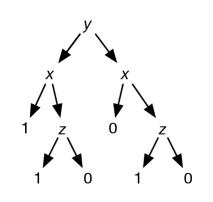
In some cases, greedy splitting does not find a simplest decision tree and it is often useful to simplify the tree resulting from the top-down algorithm, as shown in the following example.
Example 7.11.
Consider a dataset with inputs , , and and target . The target is true if is true and is true, or is false and is true. Figure 7.10 (a) shows a tree representation of this function. This tree can generate the data in the center (b).
 |
|
 |
||||||||||||||||||||||||||||||||||||
|---|---|---|---|---|---|---|---|---|---|---|---|---|---|---|---|---|---|---|---|---|---|---|---|---|---|---|---|---|---|---|---|---|---|---|---|---|---|---|
| (a) | (b) | (c) |
Although the simplest tree first splits on , splitting on provides no information; there is the same proportion of true when is true as when is false. Instead, the algorithm can split on . When is true, there is a larger proportion of true than when is false. For the case where is true, splitting on perfectly predicts the target when is true. The resulting tree is given in Figure 7.10(c). Following the paths to , this tree corresponds to being true when , which can be simplified to . This is essentially the original tree.
7.3.2 Linear Regression and Classification
Linear functions provide a basis for many learning algorithms. This section first covers regression, then considers classification.
Linear regression is the problem of fitting a linear function to a set of training examples, in which the input and target features are real numbers.
Suppose the input features, , are all real numbers (which includes the case) and there is a single target feature . A linear function of the input features is a function of the form
where is a vector (tuple) of weights, and is a special feature whose value is always 1.
Suppose is a set of examples. The mean squared loss on examples for target is the error
| (7.1) |
Consider minimizing the mean squared loss. There is a unique minimum, which occurs when the partial derivatives with respect to the weights are all zero. The partial derivative of the error in Equation 7.1 with respect to weight is
| (7.2) |
where , a linear function of the weights. The weights that minimize the error can be computed analytically by setting the partial derivatives to zero and solving the resulting linear equations in the weights (see Exercise 7.11).
Squashed Linear Functions
Consider binary classification, where the domain of the target variable is .
A linear function does not work well for such classification tasks; a learner should never make a prediction greater than 1 or less than 0. However, a linear function could make a prediction of, say, 3 for one example just to fit other examples better.
A squashed linear function is of the form
where , an activation function, is a function from the real line into some subset of the real line, such as .
A prediction based on a squashed linear function is a linear classifier.
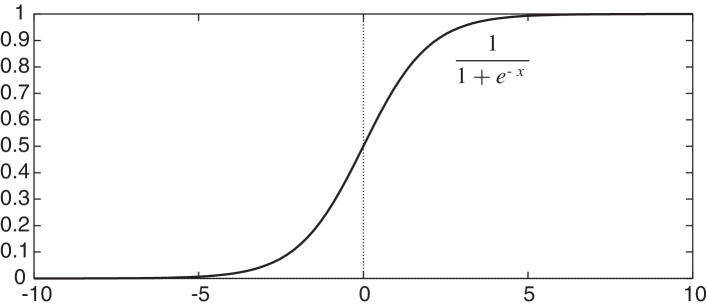
One differentiable activation function is the sigmoid or logistic function:
where , where is Euler’s number (approximately 2.718). The sigmoid function, depicted in Figure 7.11, squashes the real line into the interval , which is appropriate for classification because you would never want to make a prediction of greater than 1 or less than 0. The sigmoid function can be justified in terms of probabilities. It is also differentiable, with derivative
The problem of determining weights for the sigmoid of a linear function that minimize an error on a set of examples is called logistic regression.
The mean log loss for logistic regression is
where . To minimize this, consider weight . The partial derivative with respect to weight is
| (7.3) |
where . This is very similar to Equation 7.2, the main difference is the definition of the predicted value. Unlike Equation 7.2, this is not a linear function of the parameters (because is not linear in the parameters) and is difficult to solve analytically.
Stochastic Gradient Descent
The problem of finding a set of parameters to minimize errors is an optimization problem; see Section 4.8.
Gradient descent is an iterative method to find a local minimum of a function. To find a set of weights to minimize an error, it starts with an initial set of weights. In each step, it decreases each weight in proportion to its partial derivative:
where , the gradient descent step size, is called the learning rate. The learning rate, as well as the features and the data, is given as input to the learning algorithm. The partial derivative specifies how much a small change in the weight would change the error.
For linear regression with squared error and logistic regression with log loss, the derivatives, given in Equation 7.2 and Equation 7.3. For each of these (ignoring the constant factor of 2), gradient descent has the update
| (7.4) |
where .
A direct implementation of gradient descent does not update any weights until all examples have been considered. This can be very wasteful for large datasets. It is possible to make progress with a subset of the data. This gradient descent step takes a mean value. Often you can compute means approximately by using a random sample of examples. For example, you can get a good estimate of the mean height of a large population of people by selecting 100 or 1000 people at random and using their mean height.
Instead of using all of the data for an update, stochastic gradient descent uses a random sample of examples to update the weights. It is called stochastic because of the random sampling. Random sampling is explored more in Section 9.7. The set of examples used in each update is called a minibatch or a batch.
The stochastic gradient descent algorithm for logistic regression is shown in Figure 7.12. This returns a function, , that can be used for predictions on new examples. The algorithm collects the update for each weight for a batch in a corresponding , and updates the weights after each batch. The learning rate is assumed to be per example, and so the update needs to be divided by the batch size.
An epoch is batches, which corresponds to one pass through all of the data, on average. Epochs are useful when reporting results, particularly with different batch sizes.
Example 7.12.
Consider learning a squashed linear function for classifying the data of Figure 7.1. One function that correctly classifies the examples is
where is the sigmoid function. A function similar to this can be found with about 3000 iterations of stochastic gradient descent with a learning rate . According to this function, is true (the predicted value for example is closer to 1 than 0) if and only if is true and either or is true. Thus, in this case, the linear classifier learns the same function as the decision tree learner.
Smaller batch sizes tend to learn faster as fewer examples are required for an update. However, smaller batches may not converge to a local optimum solution, whereas more data, up to all of the data, will. To see this, consider being at an optimum. A batch containing all of the examples would end up with all of the being zero. However, for smaller batches, the weights will vary and later batches will be using non-optimal parameter settings and so use incorrect derivatives. It is common to start with small batch size and increase the batch size until convergence, or good enough performance has been obtained.
Incremental gradient descent, or online gradient descent, is a special case of stochastic gradient descent using minibatches of size 1. In this case, there is no need to store the intermediate values in , but the weights can be directly updated. This is sometimes used for streaming data where each example is used once and then discarded. If the examples are not selected at random, it can suffer from catastrophic forgetting, where it fits the later data and forgets about earlier examples.
Linear Separability
Each input feature can be seen as a dimension; features results in an -dimensional space. A hyperplane in an -dimensional space is a set of points that all satisfy a constraint that some linear function of the variables is zero. The hyperplane forms an -dimensional space. For example, in a (two-dimensional) plane, a hyperplane is a line, and in a three-dimensional space, a hyperplane is a plane. A Boolean classification is linearly separable if there exists a hyperplane where the classification is true on one side of the hyperplane and false on the other side.
The algorithm can learn any linearly separable binary classification. The error can be made arbitrarily small for arbitrary sets of examples if, and only if, the target classification is linearly separable. The hyperplane is the set of points where for the learned weights . On one side of this hyperplane, the prediction is greater than 0.5; on the other side, the prediction is less than 0.5.
Example 7.13.
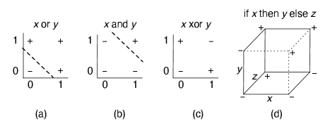
Figure 7.13 shows linear separators for “or” (a) and “and” (b). The dashed line separates the positive (true) cases from the negative (false) cases. One simple function that is not linearly separable is the exclusive-or (xor) function (c). There is no straight line that separates the positive examples from the negative examples. As a result, a linear classifier cannot represent, and therefore cannot learn, the exclusive-or function.
Suppose there are three input features , , and , each with domain , and the ground truth is the function “if then else ” (represented by in Figure 7.10). This function is depicted by the cube in Figure 7.13(d) with the origin (, , all zero) at the bottom left and the ground truth for labelled with and . This function is not linearly separable.
The following example shows what happens in gradient descent for logistic regression when the data is not linearly separable.
| 0 | 0 | 0 | 0 | 0.02 | ||
| 0 | 0 | 1 | 1 | 0.08 | 0.52 | |
| 0 | 1 | 0 | 0 | 0.08 | 0.52 | |
| 0 | 1 | 1 | 1 | 4.14 | 0.98 | |
| 1 | 0 | 0 | 0 | 0.02 | ||
| 1 | 0 | 1 | 0 | 0.49 | ||
| 1 | 1 | 0 | 1 | 0.49 | ||
| 1 | 1 | 1 | 1 | 4.14 | 0.98 | |
| (a) | (b) | |||||
Example 7.14.
Consider target from the previous example that is true if is true and is true, or is false and is true. The prediction of is not linearly separable, as shown in Figure 7.13(d) – there is no hyperplane that separates the positive and negative cases of .
After 1000 epochs of gradient descent with a learning rate of 0.05, one run found the following weights (to two decimal points):
The linear function and the prediction for each example are shown in Figure 7.14(b). Four examples are predicted reasonably well, and the other four are predicted with a value of approximately . This function is quite stable with different initializations. Increasing the number of iterations makes the predictions approach 0, 1, or 0.5.
Categorical Target Features
When the domain of the target variable is categorical with more than two values, indicator variables can be used to convert the classification to binary variables. These binary variables could be learned separately. Because exactly one of the values must be true for each example, the predicted probabilities should add to 1. One way to handle this is to learn for all-but-one value, and predict the remaining value as 1 minus the sum of the other values. This is effectively how the binary case works. However, this introduces an asymmetry in the values by treating one value differently from the other values. This is problematic because the errors for the other values accumulate, making for a poor prediction on the value treated specially; it’s even possible that the prediction for the remaining value is negative if the others sum to more than 1.
The standard alternative is to learn a linear function for each value of the target variable, exponentiate, and normalize. This has more parameters than necessary to represent the function (it is said to be over-parametrized) but treats all of the values in the same way. Suppose the target is categorical with domain represented by the tuple of values . The softmax function takes a vector (tuple) of real numbers, , and returns a vector of the same size, where the th component of the result is
This ensures that the resulting values are all positive and sum to 1, and so can be considered as a probability distribution.
Sigmoid and softmax are closely related:
where corresponds to the values and is the second component of the pair that results from the softmax. The second equality follows from multiplying the numerator and the denominator by , and noticing that . Thus, is equivalent to where the false component is fixed to be 0.
A softmax, like a sigmoid, cannot represent zero probabilities.
The generalization of logistic regression to predicting a categorical feature is called softmax regression, multinomial logistic regression, or multinomial logit. It involves a linear equation for each value in the domain of the target variable, . Suppose has domain . The prediction for example is a tuple of values, , where the th component is the prediction for and
This is typically optimized with categorical log loss.
Consider weight that is used for input for output value , and example that has :
where is 1 if is the index of the observed value, , and is the th component of the prediction. This is the predicted value minus the actual value.
To implement this effectively, you need to consider how computers represent numbers. Taking the exponential of a large number can result in a number larger than the largest number able to be represented on the computer, resulting in overflow. For example, will overflow for most modern CPUs. Taking exponentials of a large negative number can result in a number that is represented as zero, resulting in underflow. For example, results in zero on many CPUs. Adding a constant to each in a softmax does not change the value of the softmax. To prevent overflow and prevent all values from underflowing, the maximum value can be subtracted from each value, so there is always a zero, and the rest are negative. On GPUs and similar parallel hardware, often lower precision is used to represent weights, and so it becomes more important to correct for underflow and overflow.
When there is a large number of possible values, the computation of the denominator can be expensive, as it requires summing over all values. For example, in natural language, we may want to predict the next word in a text, in which case the number of values could be up to a million or more (particularly when phrases and names such as “Mahatma Gandhi” are included). In this case, it is possible to represent the prediction in terms of a binary tree of the values, forming hierarchical softmax. This implements the same function as softmax, just more efficiently for large domains.
Creating Input Features
The definitions of linear and logistic regression assume that the input features are numerical.
Categorical features can be converted into features with domain by using indicator variables, as was done for decision tree learning. This is known as a one-hot encoding.
A real-valued feature can be used directly as long as the target is a linear function of that input feature, when the other input features are fixed. If the target is not a linear function, often some transformation of the feature is used to create new features.
For ordinal features, including real-valued features, cuts can be used to define a Boolean feature from a real feature. For input feature , choose a value and use a feature that is true if , or equivalently . It is also common to use binning. Binning involves choosing a set of thresholds, , and using a feature with domain for each interval between and . Binning allows for a piecewise constant function. Constructing a feature using allows for a connected piecewise linear approximation; this is the basis of the rectified linear unit (ReLU), further investigated in the next chapter.
Designing appropriate features is called feature engineering. It is often difficult to design good features. Gradient-boosted trees use conjunctions of input features. Learning features is part of representation learning; see Chapter 8.
Artificial Intelligence: Foundations of Computational Agents, Poole
& Mackworth
Copyright © 2023, David L. Poole and Alan K. Mackworth. 
This work is licensed under a Creative Commons Attribution-NonCommercial-NoDerivatives 4.0 International License.