4 Reasoning with Constraints 4.7 Population-Based Methods 4.9 Social Impact

4.8 Optimization

Instead of just having a total assignment satisfy constraints or not, we often have a preference relation over assignments, and we want a best total assignment according to the preference.

An optimization problem is given:

•

a set of variables, each with an associated domain
•

an objective function that maps total assignments to real numbers
•

an optimality criterion, which is typically to find a total assignment that minimizes or maximizes the objective function.

The aim is to find a total assignment that is optimal according to the optimality criterion. For concreteness, we assume that the optimality criterion is to minimize the objective function. When minimizing, the function is often called the cost function, loss function, or error function.

A constrained optimization problem is an optimization problem that also has hard constraints. The set of assignments that does not violate a constraint is the set of feasible assignments. The aim is to find a feasible assignment that optimizes the objective function according to the optimality criterion.

Example 4.29.

The University of British Columbia (UBC) is one of the larger universities in Canada. It needs to schedule exams multiple times a year. Exam scheduling is a constrained optimization problem. In one term, there were 30,000 students taking exams, and 1700 course sections that needed to be scheduled into 52 time slots over 13 days, and 274 rooms. There any many courses that are divided into multiple sections, with lectures at different times, that must have exams at the same time, so there can be no simple mapping from lecture times to exam times. With the hard constraint that no student should have two exams at the same time – which seems reasonable – there are no possible exam schedules. Thus, soft constraints are needed. When an AI system started to be used for exam scheduling, the hard constraints were:

•

There must be no more than 30 conflicts for a section, where a conflict is a student that has two exams at the same time.
•

Each exam must fit into the allowable times and the allowable rooms for that exam (for the few cases where there are constraints on allowable times and rooms).
•

There cannot be more students than the room capacity in a room.
•

Each exam must go into a room that has the required room features.
•

Unrelated exams cannot share a room.
•

Cross-listed courses must have the same exam time.
•

Evening courses must have evening exams.

The soft constraints that need to be minimized include:

•

the number of conflicts
•

the number of students with two or more exams on the same day
•

the number of students with three or more exams in four consecutive time slots
•

the number of students with back-to-back exams
•

the number of students with less than eight time slots between exams
•

the preferred times for each exam
•

the preferred rooms for each exam
•

first-year exams should not be on the last two days in the Fall (to allow time for large exams to be marked before the holidays)
•

fourth-year exams should not be on the last two days in the Spring (so exams can be marked before graduation is determined).

These are not weighted equally.

One representation is that there is a time variable for each section with domain the set of possible time slots, and there is a room variable for each section, with domain the set of rooms.

This is simpler than many real-world scheduling problems as each exam only needs to be scheduled once and all of the time slots are the same length.

A huge literature exists on optimization. There are many techniques for particular forms of constrained optimization problems. For example, linear programming is the class of constrained optimization where the variables are real valued, the objective function is a linear function of the variables, and the hard constraints are linear inequalities. If the problem you are interested in solving falls into one of the classes for which there are more specific algorithms, or can be transformed into one, it is generally better to use those techniques than the more general algorithms presented here.

In a factored optimization problem, the objective function is factored into a set of soft constraints. A soft constraint has a scope that is a set of variables. The soft constraint is a function from the domains of the variables in its scope into a real number, a cost. A typical objective function is the sum of the costs of the soft constraints, and the optimality criterion is to minimize the objective function.

Example 4.30.

Suppose a number of delivery activities must be scheduled, similar to Example 4.9, but, instead of hard constraints, there are preferences on times for the activities. The values of the variables are times. The soft constraints are costs associated with combinations of times associated with the variables. The aim is to find a schedule with the minimum total sum of the costs.

Suppose variables $A$ , $C$ , $D$ , and $E$ have domain $\{1,2\}$ , and variable $B$ has domain $\{1,2,3\}$ . The soft constraints are $c_{1}$ with scope $\{A,B\}$ , $c_{2}$ with scope $\{B,C\}$ , and $c_{3}$ with scope $\{B,D\}$ . Define their extension as

$c_{1}$ : $A$ $B$ Cost 1 1 5 1 2 2 1 3 2 2 1 0 2 2 4 2 3 3 $c_{2}$ : $B$ $C$ Cost 1 1 5 1 2 2 2 1 0 2 2 4 3 1 2 3 2 0 $c_{3}$ : $B$ $D$ Cost 1 1 3 1 2 0 2 1 2 2 2 2 3 1 2 3 2 4

The constraint $c_{4}$ , with scope $\{A,C\}$ , has a cost of 3 if $A=C$ , and 0 otherwise; $c_{4}$ provides a soft constraint that $A$ and $C$ should be different.

Soft constraints can be added point-wise. The sum of two soft constraints is a soft constraint with scope that is the union of their scopes. The cost of any assignment to variables in the scope is the sum of the costs of the constraints being added on that assignment.

Example 4.31.

Consider functions $c_{1}$ and $c_{2}$ in Example 4.30. $c_{1}+c_{2}$ is a function with scope $\{A,B,C\}$ , defined point-wise. For example, $c_{1}+c_{2}$ evaluated in context $\{A{\,{=}\,}1,B{\,{=}\,}1,C{\,{=}\,}2\}$ is

	$\displaystyle(c_{1}$	$\displaystyle+c_{2})(A{\,{=}\,}1,B{\,{=}\,}1,C{\,{=}\,}2)$
		$\displaystyle=c_{1}(A{\,{=}\,}1,B{\,{=}\,}1)+c_{2}(B{\,{=}\,}1,C{\,{=}\,}2)$
		$\displaystyle=5+2=7.$

Similarly, $c_{1}+c_{2}+c_{3}$ evaluated in context $\{A{\,{=}\,}1,B{\,{=}\,}1,C{\,{=}\,}2,D{\,{=}\,}2\}$ is

	$\displaystyle(c_{1}$	$\displaystyle+c_{2}+c_{3})(A{\,{=}\,}1,B{\,{=}\,}1,C{\,{=}\,}2,D{\,{=}\,}1)$
		$\displaystyle=c_{1}(A{\,{=}\,}1,B{\,{=}\,}1)+c_{2}(B{\,{=}\,}1,C{\,{=}\,}2)+c_% {3}(B{\,{=}\,}1,D{\,{=}\,}1)$
		$\displaystyle=5+2+3=10.$

Hard constraints can be modeled as having a cost of infinity for violating a constraint. As long as the cost of an assignment is finite, it does not violate a hard constraint. An alternative is to use a large number – larger than the sum of the soft constraints could be – as the cost of violating a hard constraint. Then optimization can be used to find a solution with the fewest number of violated hard constraints and, among those, one with the lowest cost.

Optimization problems have one difficulty that goes beyond constraint satisfaction problems. It is difficult to know whether an assignment is optimal. Whereas, for a CSP, an algorithm can check whether an assignment is a solution by just considering the assignment and the constraints, in optimization problems an algorithm can only determine whether an assignment is optimal by comparing it to other assignments.

Many of the methods for solving hard constraints can be extended to optimization problems, as outlined in the following sections.

4.8.1 Systematic Methods for Discrete Optimization

When all of the variables have finite discrete domains, optimization is known as discrete optimization. In this case, it is possible to search through the space of assignments to find the least-cost assignment.

Any of the search algorithms of the previous chapter that minimize path cost can be used to search for the best solution. To do that, we need to define the optimization problem in terms of a search graph. The graph to search is defined as follows:

•

The nodes are assignments of values to some subset of the variables.
•

The neighbors of a node $n$ are obtained by selecting a variable $v a r$ that is not assigned in node $n$ and by having a neighbor for each assignment of a value to $v a r$ . The cost of the arc is the sum of the costs of the constraints that can be evaluated when $v a r$ is assigned a value.

Suppose node $n$ is the assignment $\{X_{1}{\,{=}\,}v_{1},\dots,X_{k}{\,{=}\,}v_{k}\}$ . To find the neighbors of $n$ , select a variable $Y$ that is not in the set $\{X_{1},\dots,X_{k}\}$ . For each value $y_{i}\in dom(Y)$ , where $X_{1}{\,{=}\,}v_{1},\dots,X_{k}{\,{=}\,}v_{k},Y{\,{=}\,}y_{i}$ is consistent with each of the constraints, the node $\{X_{1}{\,{=}\,}v_{1},\dots,X_{k}{\,{=}\,}v_{k},Y{\,{=}\,}y_{i}\}$ is a neighbor of $n$ . The cost of the arc is the sum of the constraints that involve only $\{X_{1},\dots,X_{k},Y\}$ that were not previously evaluated in this branch.
•

The start node is the empty assignment that does not assign a value to any variables.
•

A goal node is a node that assigns a value to every variable. Note that this only exists if the assignment is consistent with all of the constraints.

By assigning costs as soon as a soft constraint is able to be evaluated, search algorithms such as $A^{*}$ or branch and bound can be used to find a minimal solution. These methods require each arc cost to be non-negative. To achieve this, the lowest cost in each soft constraint – even if it is negative – is subtracted from each of the costs in the soft constraint. This cost then needs to be added to the cost of a final solution.

Example 4.32.

Suppose $X$ and $Y$ are variables with domain $\{0,1\}$ . The soft constraint

$X$	$Y$	Cost
0	0	$-4$
0	1	$-1$
1	0	6
1	1	5

is converted into non-negative form by subtracting $-4$ (i.e., adding 4) to each cost, so the costs range from 0 to 10, rather than from $-4$ to 6. The 4 is then subtracted from the cost of the solution.

Figure 4.12 shows the branch-and-bound search of Figure 3.14 for factored optimization. The heuristic function, $h(context,Cs)$ , is an estimate of how much the soft constraints $C s$ will cost, given $c o n t e x t$ . It can be the sum of the minimum values for the constraints in $C s$ given $c o n t e x t$ . As long as $h$ is an underestimate, the algorithm will find the optimal solution. If all of the constraints are in non-negative form, $h$ always returning zero will be an underestimate, but we can typically do much better.

1: procedure DF_branch_and_bound_const(

Vs,domain,Cs,h,{bound}_{0}

)

2: Inputs

3: variables (

V s

), domain (

d o m

), and constraints

C s

form a CSP

h

: heuristic function

{bound}_{0}

: initial depth bound (can be

\infty

if not specified)

6: Output

7: a lowest-cost total assignment with cost less than

{bound}_{0}

8: or

\bot

if there is no solution with cost less than

{bound}_{0}

9: Local

10:

{best\_asst}

: total assignment or

\bot

11:

{bound}

: non-negative real

12: procedure cbsearch(

{CVs}

{CCs}

{context}

)

13: Inputs

14:

{CVs}

is set of unassigned variables

15:

{CCs}

is set of unevaluated constraints

16:

{context}

is an assignment

17:

can\_eval\;{:}{=}\;\mbox{}\{c\in CCs\mid scope(c)\subseteq variables(context)\}

18:

rem\_Cs\;{:}{=}\;\mbox{}CCs\setminus can\_eval

19:

cost\_context\;{:}{=}\;\mbox{}\sum_{c\in can\_eval}cost(c,context)

20: if

cost\_context+h(context,rem\_Cs)<{bound}

then

21: if

CVs=\{\}

then

22:

{best\_asst}\;{:}{=}\;\mbox{}context

23:

{bound}\;{:}{=}\;\mbox{}{cost\_context}

24: else

25: select variable

var\in CVs

26: for each

val\in domain(var)

27:

{cbsearch}({CVs}\setminus\{var\},rem\_Cs,\{var=val\}\cup context)

28:

{best\_asst}\;{:}{=}\;\mbox{}\bot

29:

{bound}\;{:}{=}\;\mbox{}{bound}_{0}

30:

{cbsearch}({Vs}

{Cs}

\{\})

31: return

{best\_asst}

Figure 4.12: Depth-first branch-and-bound search for optimization

Example 4.33.

The soft constraint of Example 4.32 in non-negative form is

$X$	$Y$	Cost
0	0	0
0	1	3
1	0	10
1	1	9

In a context where $X=1$ , the heuristic value of this soft constraint is 9, the minimum cost for assignments with $X=1$ . In a context with $Y=1$ , the heuristic value is 3. The other contexts have value 0, because that is the minimum value for no assignments or for $X=0$ or $Y=0$ .

This can be made more efficient by exploiting the structure of the constraint network. In particular, if the context disconnects the constraint graph (when the assigned variables are removed), the separate components can be solved independently. This can be recognized because $C C s$ can be partitioned into sets that have no variables in $C V s$ in common. Another way to exploit structure is to cache values that have already been computed. These two refinements are explored in more detail in an analogous algorithm for probabilistic reasoning [see Section 9.5.1].

Arc consistency can be generalized to optimization problems by allowing pruning of dominated assignments. Suppose $c_{1},\dots,c_{k}$ are the soft constraints that involve $X$ . Let $c=c_{1}+\dots+c_{k}$ . Suppose $Y_{1},\dots,Y_{m}$ are the variables, other than $X$ , that are involved in $c$ . A value $v$ for variable $X$ is strictly dominated if, for all values $y_{1},\dots,y_{k}$ of $Y_{1},\dots,Y_{m}$ , some value $v^{\prime}$ of $X$ exists such that $c(X{\,{=}\,}v^{\prime},Y_{1}{\,{=}\,}y_{1},\dots,Y_{m}{\,{=}\,}y_{m})<c(X{\,{=% }\,}v,Y_{1}{\,{=}\,}y_{1},\dots,Y_{m}{\,{=}\,}y_{m})$ . Pruning strictly dominated values does not remove a minimal solution. The pruning of domains can be done repeatedly, as in the GAC algorithm.

Weakly dominated has the same definition as strictly dominated, but with “less than” replaced by “less than or equal to.” If only one solution is required, weakly dominated values can be pruned sequentially. Which weakly dominated values are removed may affect which optimal solution is found, but removing a weakly dominated value does not remove all optimal solutions.

As with arc consistency for hard constraints, pruning (strictly or weakly) dominated values may greatly simplify the problem but does not, by itself, always solve the problem. Arc consistency can be combined with domain splitting to build a search tree to find an optimal solution.

Variable elimination can also be used for soft constraints. Instead of the join, sum the factors and select the value of the eliminated variable with the minimum cost.

4.8.2 Local Search for Optimization

Local search is directly applicable to optimization problems, where the local search is used to minimize the objective function, rather than find a solution. The algorithm runs for a certain amount of time (perhaps including random restarts to explore other parts of the search space), always keeping the best assignment found thus far, and returning this as its answer.

Local search for optimization has one extra complication that does not arise when there are only hard constraints. With only hard constraints, the algorithm has found a solution when there are no conflicts. For optimization, it is difficult to determine whether the best total assignment found is the best possible solution. A local optimum is a total assignment that is at least as good, according to the optimality criterion, as any of its possible successors. A global optimum is a total assignment that is at least as good as all of the other total assignments. Without systematically searching the other assignments, the algorithm may not know whether the best assignment found so far is a global optimum or whether a better solution exists in a different part of the search space.

When using local search to solve constrained optimization problems, with both hard and soft constraints, it is often useful to allow the algorithm to violate hard constraints on the way to a solution. This is done by making the cost of violating a hard constraint some large, but finite, value.

4.8.3 Gradient Descent for Continuous Functions

Local search for optimization with continuous domains requires a more refined definition of a successor of a total assignment.

Consider a function $f(x)=y$ , where $x$ and $y$ are real numbers (e.g., $f(x)=exp(1.7*x^{2}+0.3)$ ). $f$ is continuous if a small change in $x$ can only result in a small change in $y$ . If $f$ is continuous, and $f(x)=y$ , for each $x$ and $\epsilon$ , there is an $\epsilon_{y}$ such that

f(x+\epsilon)=y+\epsilon_{y}.

Continuous means that if $\epsilon$ is small, then so is $\epsilon_{y}$ . For example, the function $int(x)$ that returns the largest integer smaller than $x$ is not continuous.

$f$ is smooth if it doesn’t have any abrupt angles. For example, $f(x)=max(x,0)$ is continuous but not smooth. A continuous and smooth function can be approximated at a point by a linear function of $\epsilon$ :

f(x+\epsilon)=f(x)+\epsilon*\delta.

This approximation gets better, the smaller that $\epsilon$ is. Solving for $\delta$ gives $\delta=(f(x+\epsilon)-f(x))/\epsilon$ . For a continuous and smooth function, as $\epsilon$ gets closer to zero, this ratio gets closer to a value called the derivative of $f$ at $x$ , written $(\frac{d}{dx}f)(x)$ . Thus, $\frac{d}{dx}f$ is the function that returns the slope of $f$ at any point. You do not need to know how to derive the derivative; modern tools are good at automatically differentiating any function that is made up of addition, subtraction, exponentiation, and may other functions.

If $f$ is a function of one variable, the derivative is sometimes written $f^{\prime}$ . The function $f(v)+x*f^{\prime}(v)$ is called the tangent of $f$ at $v$ . The derivative of $f$ at a point gives the slope of the tangent at that point. The tangent of a function at $v$ approximates the function near $v$ .

Refer to caption — Figure 4.13: Derivatives and gradient decent

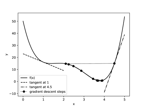
Example 4.34.

Consider the function $f(x)=2*(x-1.3)*(x-1.5)*(x-2)*(x-4.5)+15$ plotted in Figure 4.13. The tangents of $f$ at $1$ and $4.5$ are shown. Notice how they form a good approximation to the function close to these points, even though they may be a poor approximation at further points.

A (small) step in the direction of the derivative will increase the value unless the derivative is zero. A small step in the opposite direction will reduce the value. To find a minimum, gradient descent takes steps in the direction of the negative of the gradient. Gradient descent is like walking downhill and always taking a step in the direction that is locally downward. The successor of a total assignment is a step downhill, where the steps become bigger as the slope becomes steeper.

To minimize $f(x)$ , where $x$ is a real-valued variable with current value of $v$ , the next value

v-\eta*\left(\frac{df}{dx}\right)(v)

where $\eta$ is the step size determines how big a step to take. The algorithm is sensitive to the step size. If $\eta$ is too large, the algorithm can overshoot the minimum. If $\eta$ is too small, progress becomes very slow.

Example 4.35.

Consider finding the minimum value for a function $f(x)$ shown in Figure 4.13. Suppose the step size is $0.05$ and gradient descent starts at $x=4.5$ . The derivative is positive, so it steps to the left. Here it overshoots the minimum and the next position is $x=2.1$ , where the derivative is negative and has a smaller absolute value, so it takes a smaller step to the right. The steps are shown as the dotted trajectory in Figure 4.13. It eventually finds a point close to the minimum. At that point the derivative is close to zero and so it makes very small steps.

If the step size was slightly larger, it could step into the shallow local minimum between 1.3 and 1.5, where the derivative is close to zero, and would be stuck there. If it took an even larger step, it might end up with $x$ close to zero or negative, in which case the derivative is larger in magnitude and will then step to a value greater than 4.5, and eventually diverges.

If the step size was much smaller, it might take a longer time to get to the local minimum. There is nothing special about 0.05. For example, if the $y$ values were 10 times as much, a step size of 0.005 would give the same behavior.

For multidimensional optimization, when there are many variables, the partial derivative of a function with respect to a variable is the derivative of the function with the other variables fixed. We write $\frac{\partial f}{\partial x}$ to be the derivative of $f$ , with respect to variable $x$ , with the other variables fixed.

Gradient descent takes a step in each direction proportional to the partial derivative of that direction. If $\left<x_{1},\ldots,x_{n}\right>$ are the variables that have to be assigned values, a total assignment corresponds to a tuple of values $\left<v_{1},\ldots,v_{n}\right>$ . Assume that the evaluation function to be minimized, $h$ , is continuous and smooth. The successor of the total assignment $\left<v_{1},\ldots,v_{n}\right>$ is obtained by moving in each direction in proportion to the slope of $h$ in that direction. The new value for $X_{i}$ is

v_{i}-\eta*\left(\frac{\partial h}{\partial x_{i}}\right)(v_{1},\ldots,v_{n})

where $\eta$ is the step size.

Gradient descent and variants are used for parameter learning; some large language models have over $10^{12}$ parameters to be optimized. There are many variants of this algorithm. For example, instead of using a constant step size, the algorithm could do a binary search to determine a locally optimal step size. See Section 8.2 for variants used in modern neural networks.

For smooth functions, where there is a minimum, if the step size is small enough, gradient descent will converge to a local minimum. If the step size is too big, it is possible that the algorithm will diverge. If the step size is too small, the algorithm will be very slow. If there is a unique local minimum which is the global minimum, gradient descent, with a small enough step size, will converge to that global minimum. When there are multiple local minima, not all of which are global minima, it may need to search to find a global minimum, for example by doing a random restart or a random walk. These are not guaranteed to find a global minimum unless the whole search space is exhausted, but are often as good as we can get. The algorithms that power modern deep learning algorithms are described Section 8.2; these adapt the step size for each dimension.

Artificial Intelligence 3E