Artificial
Intelligence 3E
foundations of computational agents
4.6 Local Search
The preceding algorithms systematically search the space of assignments of values to variables. If the space is finite, they will either find a solution or report that no solution exists. Unfortunately, many spaces are too big for systematic search and are possibly even infinite. In any reasonable time, systematic search will have failed to consider enough of the space to give any meaningful results. This section and the next consider methods intended to work in these very large spaces. The methods do not systematically search the whole search space but they are designed to find solutions quickly on average. They do not guarantee that a solution will be found even if one exists, and so they are not able to determine that no solution exists. They are often the method of choice for applications where solutions are known to exist or are very likely to exist.
Local search methods start with a total assignment of a value to each variable and try to improve this assignment iteratively by taking improving steps, by taking random steps, or by restarting with another total assignment. Many different local search techniques have been proposed. Understanding when these techniques work for different problems forms the focus of a number of research communities, in both operations research and AI.
A generic local search algorithm is given in Figure 4.8. It maintains a total assignment in the dictionary , which has the variables as the keys. Each iteration of the outer (repeat) loop is called a try. The first for each loop (line 11) assigns a random value to each variable. The first time it is executed is called a random initialization. At subsequent times it is a random restart. An alternative to random assignment is to use an informed guess, utilizing heuristic or prior knowledge, which is then iteratively improved.
The while loop (line 13 to line 15) does a local search, or a walk, through the assignment space. It considers a set of possible successors of the total assignment , and selects one to be the next total assignment. In Figure 4.8, the possible successors of a total assignment are those assignments that differ in the assignment of a single variable.
This walk through assignments continues until either a satisfying assignment is found and returned or the condition is true, in which case the algorithm either does a random restart, starting again with a new assignment, or terminates with no solution found. A common case is that becomes true after a certain number of steps.
An algorithm is complete if it guarantees to find an answer whenever there is one. This algorithm can be complete or incomplete, depending on the selection of variable and value, and the and conditions.
One version of this algorithm is random sampling. In random sampling, the stopping criterion always returns true so that the while loop from line 13 is never executed. Random sampling keeps picking random assignments until it finds one that satisfies the constraints, and otherwise it does not halt. Random sampling is complete in the sense that, given enough time, it guarantees that a solution will be found if one exists, but there is no upper bound on the time it may take. It is typically very slow. The efficiency depends on the product of the domain sizes and how many solutions exist.
Another version is a random walk when is always false, and the variable and value are selected at random. Thus there are no random restarts, and the while loop is only exited when it has found a satisfying assignment. Random walk is also complete in the same sense as random sampling. Each step takes less time than resampling all variables, but it can take more steps than random sampling, depending on how the solutions are distributed. When the domain sizes of the variables differ, a random walk algorithm can either select a variable at random and then a value at random, or select a variable–value pair at random. The latter is more likely to select a variable when it has a larger domain.
4.6.1 Iterative Best Improvement
Iterative best improvement is a local search algorithm that selects a variable and value on line 14 of Figure 4.8 that most improves some evaluation function. If there are several possible successors that most improve the evaluation function, one is chosen at random. When the aim is to minimize a function, this algorithm is called greedy descent. When the aim is to maximize a function, this is called hill climbing or greedy ascent. We only consider minimization; to maximize a quantity, you can minimize its negation.
Iterative best improvement requires a way to evaluate each total assignment. For constraint satisfaction problems, a common evaluation function is the number of constraints that are violated. A violated constraint is called a conflict. With the evaluation function being the number of conflicts, a solution is a total assignment with an evaluation of zero. Sometimes this evaluation function is refined by weighting some constraints more than others.
A local optimum is an assignment such that no possible successor improves the evaluation function. This is also called a local minimum in greedy descent, or a local maximum in greedy ascent. A global optimum is an assignment that has the best value out of all assignments. All global optima are local optima, but there can be many local optima that are not a global optimum.
If the heuristic function is the number of conflicts, a satisfiable CSP has a global optimum with a heuristic value of 0, and an unsatisfiable CSP has a global optimum with a value above 0. If the search reaches a local minimum with a value above 0, you do not know if it is a global minimum (which implies the CSP is unsatisfiable) or not.
Example 4.24.
Consider the delivery scheduling in Example 4.9. Suppose greedy descent starts with the assignment , , , , . This assignment has an evaluation of 3, because it violates , , and . One possible successor with the minimal evaluation has with an evaluation of because only is unsatisfied. This assignment is selected. This is a local minimum. One possible successor with the fewest conflicts can be obtained by changing to , which has an evaluation of 2. It can then change to , with an evaluation of , and then change to , with an evaluation of 0, and a solution is found.
The following gives a trace of the assignments through the walk:
| Evaluation | |||||
|---|---|---|---|---|---|
| 2 | 2 | 3 | 2 | 1 | 3 |
| 2 | 4 | 3 | 2 | 1 | 1 |
| 2 | 4 | 3 | 4 | 1 | 2 |
| 4 | 4 | 3 | 4 | 1 | 2 |
| 4 | 2 | 3 | 4 | 1 | 0 |
Different initializations, or different choices when multiple assignments have the same evaluation, give different sequences of assignments to the variables and possibly different results.
Iterative best improvement considers the best successor assignment even if it is equal to or even worse than the current assignment. This means that if there are two or more assignments that are possible successors of each other and are all local, but not global, optima, it will keep moving between these assignments, and never reach a global optimum. Thus, this algorithm is not complete.
4.6.2 Randomized Algorithms
Iterative best improvement randomly picks one of the best possible successors of the current assignment, but it can get stuck in local minima that are not global minima.
Randomness can be used to escape local minima that are not global minima in two main ways:
-
•
random restart, in which values for all variables are chosen at random; this lets the search start from a completely different part of the search space
-
•
random steps, in which some random selections of variable and/or value are interleaved with the optimizing steps; with greedy descent, this process allows for upward steps that may enable random walk to escape a local minimum that is not a global minimum.
A random step is a cheap local operation only affecting a single variable, whereas a random restart is a global operation affecting all variables. For problems involving a large number of variables, a random restart can be quite expensive.
A mix of iterative best improvement with random steps is an instance of a class of algorithms known as stochastic local search.
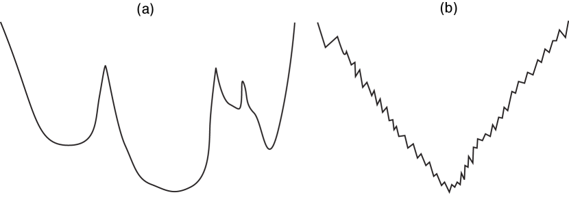
Unfortunately, it is very difficult to visualize the search space to understand which algorithms work because there are often thousands or millions of dimensions (variables), each with a discrete, or even continuous, set of values. Some intuitions can be gleaned from lower-dimensional problems. Consider the two one-dimensional search spaces in Figure 4.9, where the objective is to find the minimum value. Suppose that a possible successor is obtained by a small step, either left or right of the current position. To find the global minimum in the search space (a), one would expect the greedy descent with random restart after a local optimum has been found to find the optimal value quickly. Once a random choice has found a point in the deepest valley, greedy descent quickly leads to the global minimum. One would not expect a random walk to work well in this example, because many random steps are required to exit one of the local, but not global, minima. However, for search space (b), a random restart quickly gets stuck on one of the jagged peaks and does not work very well. However, a random walk combined with greedy descent enables it to escape these local minima. A few random steps may be enough to escape a local minimum. Thus, one may expect that a random walk would work better in this search space.
Because it is difficult to determine which method would work best from examining the problem, practitioners evaluate many methods to see which one works well in practice for the particular problem. It is even possible that different parts of the search space have different characteristics. Some of the most efficient methods use algorithm portfolios – sets of algorithms, together with a learned function that, given a problem, chooses an appropriate algorithm from the portfolio.
4.6.3 Local Search Variants
There are many variants of iterative best improvement with randomness.
If the variables have small finite domains, a local search algorithm can consider all other values of the variable when considering the possible successors. If the domains are large, the cost of considering all the other values may be too high. An alternative is to consider only a few other values, often the close values, for one of the variables. Sometimes quite sophisticated methods are used to select an alternative value.
As presented, the local search has no memory. It does not remember anything about the search as it proceeds. A simple way to use memory to improve a local search is to use tabu search, which prevents recently changed variable assignments from being changed again. The idea is, when selecting a variable to change, not to select a variable that was changed in the last steps for some integer , called the tabu tenure. If is small, tabu search can be implemented by having a list of the recently changed variables. If is larger, it can be implemented by including, for each variable, the step at which the variable got its current value. Tabu search prevents cycling among a few assignments. The tabu tenure is one of the parameters that can be optimized. A tabu list of size 1 is equivalent to not allowing the same assignment to be immediately revisited.
Algorithms differ in how much work they require to guarantee the best improvement step. At one extreme, an algorithm can guarantee to select one of the new assignments with the best improvement out of all possible successors. At the other extreme, an algorithm can select a new assignment at random and reject the assignment if it makes the situation worse. It is often better to make a quick choice than to spend a lot of time making the best choice. Which of these methods works best is, typically, an empirical question; it is difficult to determine theoretically whether large slow steps are better than small quick steps for a particular problem domain. There are many possible variants of which successor to select, some of which are explored in the next sections.
Most Improving Step
The most improving step method always selects a variable–value pair that makes the best improvement. If there are many such pairs, one is chosen at random.
The naive way of implementing most improving step is, given the current total assignment, , to linearly scan the variables, and for each variable and for each value in the domain of (other than the value of in ), evaluate the assignment but with . Then select one of the variable–value pairs that results in the lowest evaluation. One step requires evaluations of constraints, where is the number of variables, is the domain size, and is the number of constraints for each variable.
A more sophisticated alternative is to have a priority queue of variable–value pairs with associated weights. For each variable , and each value in the domain of such that is not assigned to in , the pair is in the priority queue with weight the evaluation of , but with minus the evaluation of . This weight depends on values assigned to and the other variables in the constraints involving in the constraint, but does not depend on the values assigned to other variables. At each stage, the algorithm selects a variable–value pair with minimum weight, which gives a successor with the biggest improvement. Once a variable has been given a new value, the weights of all variable–value pairs that participate in a constraint that has been made satisfied or been made unsatisfied by the new assignment to must have their weights reassessed and, if changed, they need to be reinserted into the priority queue.
The size of the priority queue is , where is the number of variables and is the average domain size. To insert or remove an element takes time . The algorithm removes one element from the priority queue, adds another, and updates the weights of at most variables, where is the number of constraints per variable and is the number of variables per constraint. The complexity of one step of this algorithm is , where is the number of variables, is the average domain size, and is the number of constraints per variable. This algorithm spends much time maintaining the data structures to ensure that the most improving step is taken at each time.
Two-Stage Choice
An alternative is to first select a variable and then select a value for that variable. The two-stage choice algorithm maintains a priority queue of variables, weighted by the number of conflicts (unsatisfied constraints) in which each variable participates. At each time, the algorithm selects a variable that participates in the maximum number of conflicts. Once a variable has been chosen, it can be assigned either a value that minimizes the number of conflicts or a value at random. For each constraint that becomes true or false as a result of this new assignment, the other variables participating in the constraint must have their weight re-evaluated.
The complexity of one step of this algorithm is , where is the number of variables and is the number of constraints per variable, and is the number of variables per constraint. Compared to selecting the best variable–value pair, this does less work for each step and so more steps are achievable for any given time period. However, the steps tend to give less improvement, giving a trade-off between the number of steps and the complexity per step.
Any Conflict
Instead of choosing the best variable, an even simpler alternative is to select any variable participating in a conflict. A variable that is involved in a conflict is a conflicting variable. In the any-conflict algorithm, at each step, one of the conflicting variables is selected at random. The algorithm assigns to the chosen variable one of the values that minimizes the number of violated constraints or a value at random.
There are two variants of this algorithm, which differ in how the variable to be modified is selected:
-
•
In the first variant, a conflict is chosen at random, and then a variable that is involved in the conflict is chosen at random.
-
•
In the second variant, a variable that is involved in a conflict is chosen at random.
These differ in the probability that a variable in a conflict is chosen. In the first variant, the probability a variable is chosen depends on the number of conflicts it is involved in. In the second variant, all of the variables that are in conflicts are equally likely to be chosen.
Each of these algorithms requires maintaining data structures that enable a variable to be quickly selected at random. The data structure needs to be maintained as variables change their values. The first variant requires a set of conflicts from which a random element is selected, such as a binary search tree. The complexity of one step of this algorithm is thus , where is the number of constraints per variable and is the number of constraints, because in the worst case constraints may need to be added or removed from the set of conflicts.
Simulated Annealing
The last method maintains no data structure of conflicts; instead, it picks a variable and a new value for that variable at random and either rejects or accepts the new assignment.
Annealing is a metallurgical process where molten metals are slowly cooled to allow them to reach a low-energy state, making them stronger. Simulated annealing is an analogous method for optimization. It is typically described in terms of thermodynamics. The random movement corresponds to high temperature; at low temperature, there is little randomness. Simulated annealing is a stochastic local search algorithm where the temperature is reduced slowly, starting from approximately a random walk at high temperature, eventually becoming pure greedy descent as it approaches zero temperature. The randomness should allow the search to jump out of local minima and find regions that have a low heuristic value, whereas the greedy descent will lead to local minima. At high temperatures, worsening steps are more likely than at lower temperatures.
Like the other local search methods, simulated annealing maintains a current total assignment. At each step, it picks a variable at random, then picks a value for that variable at random. If assigning that value to the variable does not increase the number of conflicts, the algorithm accepts the assignment of that value to the variable, resulting in a new current assignment. Otherwise, it accepts the assignment with some probability, depending on the temperature and how much worse the new assignment is than the current assignment. If the change is not accepted, the current assignment is unchanged.
Suppose is the current total assignment and is the evaluation of assignment to be minimized. For constraint solving, is typically the number of conflicts of . Simulated annealing selects a possible successor at random, which gives a new assignment . If , it accepts the assignment and becomes the new assignment. Otherwise, the new assignment is accepted randomly, using a Gibbs distribution or Boltzmann distribution, with probability
where is a positive real-valued temperature parameter. This is only used when , and so the exponent is always negative. If is close to , the assignment is more likely to be accepted. If the temperature is high, the exponent will be close to zero, and so the probability will be close to one. As the temperature approaches zero, the exponent approaches , and the probability approaches zero.
| Temperature | Probability of Acceptance | |||
|---|---|---|---|---|
| 1-worse | 2-worse | 3-worse | ||
| 10 | 0.9 | 0.82 | 0.74 | |
| 1 | 0.37 | 0.14 | 0.05 | |
| 0 | .25 | 0.018 | 0.0003 | 0.000006 |
| 0 | .1 | 0.00005 | ||
Table 4.1 shows the probability of accepting worsening steps at different temperatures. In this figure, -worse means that . For example, if the temperature is 10, a change that is one worse (i.e., if ) will be accepted with probability ; a change that is two worse will be accepted with probability . If the temperature is 1, accepting a change that is one worse will happen with probability . If the temperature is 0.1, a change that is one worse will be accepted with probability . At this temperature, it is essentially only performing steps that improve the value or leave it unchanged.
If the temperature is high, as in the case, the algorithm tends to accept steps that only worsen a small amount; it does not tend to accept very large worsening steps. There is a slight preference for improving steps. As the temperature is reduced (e.g., when ), worsening steps, although still possible, become much less likely. When the temperature is low (e.g., ), it is very rare that it selects a worsening step.
Simulated annealing requires an annealing schedule, which specifies how the temperature is reduced as the search progresses. Geometric cooling is one of the most widely used schedules. An example of a geometric cooling schedule is to start with a temperature of 10 and multiply by 0.99 after each step; this will give a temperature of 0.07 after 500 steps. Finding a good annealing schedule is an art, and depends on the problem.
4.6.4 Evaluating Randomized Algorithms
It is difficult to compare randomized algorithms when they give a different result and a different run time each time they are run, even for the same problem. It is especially difficult when the algorithms sometimes do not find an answer; they either run forever or must be stopped at an arbitrary point.
Unfortunately, summary statistics, such as the mean or median run time, are not very useful. For example, comparing algorithms on the mean run time requires deciding how to average in unsuccessful runs, where no solution was found. If unsuccessful runs are ignored in computing the average, an algorithm that picks a random assignment and then stops would be the best algorithm; it does not succeed very often, but when it does, it is very fast. Treating the non-terminating runs as having infinite time means all algorithms that do not find a solution will have infinite averages. A run that has not found a solution will need to be terminated. Using the time it was terminated in the average is more of a function of the stopping time than of the algorithm itself, although this does allow for a crude trade-off between finding some solutions fast versus finding more solutions.
If you were to compare algorithms using the median run time, you would prefer an algorithm that solves the problem 51% of the time but very slowly over one that solves the problem 49% of the time but very quickly, even though the latter is more useful. The problem is that the median (the 50th percentile) is just an arbitrary value; you could just as well consider the 47th percentile or the 87th percentile.
One way to visualize the run time of an algorithm for a particular problem is to use a run-time distribution, which shows the variability of the run time of a randomized algorithm on a single problem instance. The -axis represents either the number of steps or the run time. The -axis shows, for each value of , the number of runs, or the proportion of the runs, solved within that run time or number of steps. Thus, it provides a cumulative distribution of how often the problem was solved within some number of steps or run time. For example, you can find the run time of the 30th percentile of the runs by finding the -value that maps to 30% on the -scale. The run-time distribution can be plotted (or approximated) by running the algorithm for a large number of times (say, 100 times for a rough approximation or 1000 times for a reasonably accurate plot) and then by sorting the runs by run time.
Example 4.25.
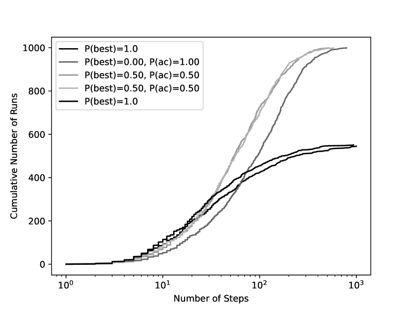
Five empirically generated run-time distributions for the CSP of Figure 4.5 are shown in Figure 4.10. On the -axis is the number of steps, using a logarithmic scale. On the -axis is the number of instances that were successfully solved out of 1000 runs. This shows five run-time distributions on the same problem instance.
The two dark lines (labeled ) use the same settings, and show an example of the variability of using 1000 runs. These solved the problem 20% of the time in 19 or fewer steps, but only solved the problem in around 55% of the cases.
The any-conflict case (labeled , ) took 32 steps to solve 20% of the runs, but managed to solve in all runs, taking up to 784 steps.
The other two cases, which chose the best node with probability 0.5 and otherwise chose a constraint in any conflict, solved all of the problems. Again these two cases used the same settings and show the variability of the experiment.
This only compares the number of steps; the time taken would be a better evaluation but is more difficult to measure for small problems and depends on the details of the implementation. The any-conflict algorithm takes less time than maintaining the data structures for finding a most-improving variable choice. The other algorithms that need to maintain the same data structures take a similar time per step.
One algorithm strictly dominates another for this problem if its run-time distribution is completely to the left (and above) the run-time distribution of the second algorithm. Often two algorithms are incomparable under this measure. Which algorithm is better depends on how much time an agent has before it needs to use a solution or how important it is to actually find a solution.
Example 4.26.
In the run-time distributions of Figure 4.10, the probabilistic mix , dominated . For any number of steps, it solved the problem in more runs.
This example was very small, and the empirical results here may not reflect performance on larger or different problems.
4.6.5 Random Restart
It may seem like a randomized algorithm that only succeeds, say, 20% of the time is not very useful if you need an algorithm to succeed, say, 99% of the time. However, a randomized algorithm that succeeds some of the time can be extended to an algorithm that succeeds more often by running it multiple times, using a random restart, and reporting any solution found.
Whereas a random walk, and its variants, are evaluated empirically by running experiments, the performance of random restart can also be predicted ahead of time, because the runs following a random restart are independent of each other.
A randomized algorithm for a problem that has a solution, and succeeds with probability independently each time, that is run times or until a solution is found, will find a solution with probability . It fails to find a solution if it fails for each retry, and each retry is independent of the others.
For example, an algorithm that succeeds with probability tried 5 times will find a solution around 96.9% of the time; tried 10 times it will find a solution 99.9% of the time. If each run succeeded with a probability , running it 10 times will succeed 65% of the time, and running it 44 times will give a 99% success rate. It is also possible to run these in parallel.
A run-time distribution allows us to predict how the algorithm will work with random restart after a certain number of steps. Intuitively, a random restart will repeat the lower left corner of the run-time distribution, suitably scaled down, at the stage where the restart occurs. A random restart after a certain number of greedy descent steps will make any algorithm that sometimes finds a solution into an algorithm that always finds a solution, given that one exists, if it is run for long enough.
Example 4.27.
In the distribution of Figure 4.10, greedy search () solved more problems in the first 10 steps, after which it is not as effective as any-conflict search or a probabilistic mix. This may lead you to try to suggest using these settings with a random restart after 10 steps. This does, indeed, dominate the other algorithms for this problem instance, at least in terms of the number of steps (counting a restart as a single step). However, because the random restart is an expensive operation, this algorithm may not be the most efficient. This also does not necessarily predict how well the algorithm will work in other problem instances.
A random restart can be expensive if there are many variables. A partial restart randomly assigns just some not all of the variables, say 100 variables, or 10% of the variables, to move to another part of the search space. While this is often effective, the above theoretical analysis does not work because the partial restarts are not independent of each other.
Artificial Intelligence: Foundations of Computational Agents, Poole
& Mackworth
Copyright © 2023, David L. Poole and Alan K. Mackworth. 
This work is licensed under a Creative Commons Attribution-NonCommercial-NoDerivatives 4.0 International License.