Artificial
Intelligence 3E
foundations of computational agents
8.2 Improved Optimization
Stochastic gradient descent is the workhorse for parameter learning in neural networks. However, setting the step size is challenging. The structure of the multidimensional search space – the error as a function of the parameter settings – is complex. For a model with, say, a million parameters, the search space has a million dimensions, and the local structure can vary across the dimensions.
One particular challenge is a canyon, where there is a U-shaped error function in one dimension and another dimension has a downhill slope. Another is a saddle point, where a minimum in one dimension meets a maximum of another. Close to a saddle point, moving along the dimension that is at a maximum, there is a canyon, so a way to handle canyons should also help with saddle points.
Example 8.4.
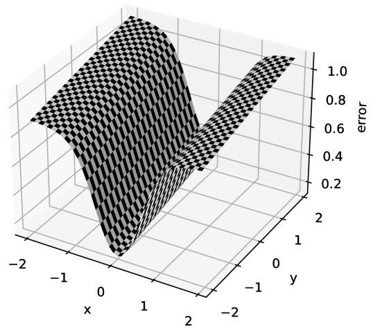
Figure 8.6 depicts a canyon with two parameters. The error is plotted as a function of parameters and . In the -direction the error has a steep valley, but in the -direction there is a gentle slope. A large step size would keep jumping from side-to-side of the valley, perhaps diverging. A small step size is needed for the -value to decrease. However, a small step size in the -direction means very slow convergence. Ideally, you would like small steps in the -direction and large steps in the -direction.
There are two main approaches to adapting step size to handle canyons and related problems. Both have a separate step size for each parameter. They can be combined. The intuition behind each is:
-
•
If the sign of the gradient doesn’t change, the step size can be larger; if the sign keeps changing, the step size should be smaller.
-
•
Each weight update should follow the direction of the gradient, and the magnitude should depend on whether the gradient is more or less than its historic value.
8.2.1 Momentum
The momentum for each parameter acts like a velocity of the update for each parameter, with the standard stochastic gradient descent update acting like an acceleration. The momentum acts as the step size for the parameter. It is increased if the acceleration is the same sign as the momentum and is decreased if the acceleration is the opposite sign.
To implement momentum, a velocity is stored for each weight . Hyperparameter , with , specifies how much of the momentum should be used for each batch. The method for in Figure 8.3 becomes
The change in weight is not necessarily in the direction of the gradient of the error, because the momentum might be too great.
The value of affects how much the step size can increase. Common values for are 0.5, 0.9, and 0.99. If the gradients have the same value, the step size will approach times the step size without momentum. If is 0.5, the step size could double. If is 0.9, the step size could increase up to 10 times, and allows the step size to increase by up to 100 times.
Example 8.5.
Consider the error surface of Figure 8.6, described in Example 8.4. In the -direction, the gradients are consistent, and so momentum will increase the step size, up to times. In the -direction, as the valley is crossed, the sign of the gradient changes, and the momentum, and so the steps, get smaller. This means that it eventually makes large steps in the -direction, but small steps in the -direction, enabling it to move down the canyon.
As well as handling canyons, momentum can average out noise due to the batches not including all the examples.
8.2.2 RMS-Prop
RMS-Prop (root mean squared propagation) is the default optimizer for the Keras deep learning library. The idea is that the magnitude of the change in each weight depends on how (the square of) the gradient for that weight compares to its historic value, rather than depending on the absolute value of the gradient. For each weight, a rolling average of the square of the gradient is maintained. This is used to determine how much the weight should change. A correction to avoid numeric instability of dividing by approximately zero is also used.
The hyperparameters for RMS-Prop are the learning rate (with a default of in Keras), (with a default of in Keras) that controls the time horizon of the rolling average, and (defaults to in Keras) to ensure numerical stability. The algorithm below maintains a rolling average of the square of the gradient for in . The method for in Figure 8.3 becomes
To understand the algorithm, assume the value of is initially much bigger than , so that .
-
•
When , the ratio is approximately 1 or , depending on the sign of , so the magnitude of the change in weight is approximately .
-
•
When is bigger than , the error has a larger magnitude than its historical value, is increased, and the step size increases.
-
•
When is smaller than , the value is decreased, and the step size decreases. When a local minimum is approached, the values of and become smaller than the magnitude of , so the updates are dominated by , and the step is small.
RMS-Prop only affects the magnitude of the step; the direction of change of is always opposite to .
Example 8.6.
Consider the error surface of Figure 8.6, described in Example 8.4. In the -direction, the gradients are consistent, and so will be approximately the same as the square root of , the average squared value of , and so, assuming is much greater than , the change in will have magnitude approximately .
In the -direction, it might start with a large gradient, but when it encounters a flatter region, becomes less than the rolling average , so the step size is reduced. As for that parameter becomes very small, the steps get very small because they are less than their historical value, eventually becoming dominated by .
8.2.3 Adam
Adam, for “adaptive moments”, is an optimizer that uses both momentum and the square of the gradient, similar to RMS-Prop. It also uses corrections for the parameters to account for the fact that they are initialized at 0, which is not a good estimate to average with. Other mixes of RMS-Prop and momentum are also common.
It takes as hyperparameters: learning-rate (), with a default of 0.001; , with a default of 0.9; , with a default of 0.999; and , with a default of . (Names and defaults are consistent with Keras.)
Adam takes the gradient, , for the weight and maintains a rolling average of the gradient in , a rolling average of the square of the gradient in , and the step number, . These are all initialized to zero. To implement Adam, the method for in Figure 8.3 becomes:
The weight update step (line 7) is like RMS-Prop but uses instead of the gradient in the numerator, and corrects it by dividing by . Note that and are the names of the parameters, but the superscript is the power. In the first update, when , is equal to ; it corrects subsequent updates similarly. It also corrects by dividing by . Note that is inside the square root in RMS-Prop, but is outside in Adam.
8.2.4 Initialization
For convergence, it helps to normalize the input parameters, and sensibly initialize the weights.
For example, consider a dataset of people with features including height (in cm), the number of steps walked in a day, and a Boolean which specifies whether they have passed high school. These use very different units, and might have very different utility in predictions. To make it learn independently of the units, it is typical to normalize each real-valued feature, by subtracting the mean, so the result has a mean of 0, and dividing by the standard deviation, so the result has a standard deviation and variance of 1. Each feature is scaled independently.
Categorical inputs are usually represented as indicator variables, so that categorical variable with domain is represented as inputs, . An input example with is represented with and every other . This is also called a one-hot encoding.
The weights for the linear functions in hidden layers cannot all be assigned the same value, otherwise they will converge in lock-step, never learning different features. If the parameters are initialized to the same value, all of the units at one layer will implement the same function. Thus they need to be initialized to random values. In Keras, the default initializer is the Glorot uniform initializer, which chooses values uniformly in the interval between , where is the number of inputs and is the number of outputs for the linear function. This has a theoretical basis and tends to work well in practice for many cases. The biases (the weights multiplied by input unit 1) are typically initialized to 0.
For the output units, the bias can be initialized to the value that would predict best when all of the other inputs are zero. This is the mean for regression, or the inverse-sigmoid of the empirical probability for binary classification. The other output weights can be set to 0. This allows the gradient descent to learn the signal from the inputs, and not the background average.
Artificial Intelligence: Foundations of Computational Agents, Poole
& Mackworth
Copyright © 2023, David L. Poole and Alan K. Mackworth. 
This work is licensed under a Creative Commons Attribution-NonCommercial-NoDerivatives 4.0 International License.