8 Neural Networks and Deep Learning 8 Neural Networks and Deep Learning 8.2 Improved Optimization

8.1 Feedforward Neural Networks

There are many different types of neural networks. A feedforward neural network implements a prediction function given inputs $x$ as

f(x)=f_{n}(f_{n-1}(\dots f_{2}(f_{1}(x)))).

(8.1)

Each function $f_{i}$ maps a vector (array or list) of values into a vector of values. The function $f_{i}$ is the $i$ th layer. The number of functions composed, $n$ , is the depth of the neural network. The last layer, $f_{n}$ , is the output layer. The other layers are called hidden layers. Sometimes the input, $x$ , is called the input layer. Each component of the output vector of a layer is called a unit. The “deep” in deep learning refers to the depth of the network.

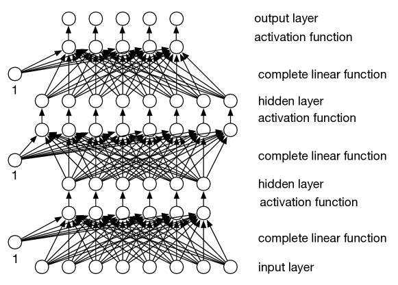
Refer to caption — Figure 8.1: A feedforward neural network of depth three. On the bottom is the input layer which is fed the input features. On the top is the output layer that makes predictions for the target features. In each dense linear function, the leftmost input is clamped at 1, and there is a parameter for each arc. The activation function is applied to each value

In a feedforward network, each layer $f_{i}$ is a linear function with learnable parameters of each output given the input, similar to linear or logistic regression, followed by a nonlinear activation function, $\phi$ . The linear function takes a vector $i n$ of values for the inputs to the layer (and, as in linear regression, an extra constant input that has value “1”), and returns a vector $o u t$ of output values, so that

out[j]=\phi(\sum_{k}in[k]*w[k,j])

for a two-dimensional array $w$ of weights. The weight associated with the extra 1 input is the bias. There is a weight $w[i,j]$ for each input–output pair of the layer, plus a bias for each output. The outputs of one layer are the inputs to the next. See Figure 8.1.

The activation function $\phi$ for the hidden layers is a nonlinear function. If it is a linear function (or the identity), the layer is redundant as a linear function of a linear function is another linear function. An activation function should be (almost everywhere) differentiable so that methods based on gradient descent work.

A common activation function for hidden layers is the rectified linear unit (ReLU): defined by $\phi(x)=max(0,x)$ . That is

\phi(x)=\left\{\begin{array}[]{ll}0&\mbox{ if }x<0\\ x&\mbox{ if }x\geq 0.\end{array}\right.

$\phi$ has derivative 0 for $x<0$ and 1 for $x>0$ . Although it does not have a derivative for $x=0$ , assume the derivative is 0. If all the hidden layers use ReLU activation, the network implements a piecewise linear function.

The activation function for the output layer depends on the type of the output $y$ and the error function (loss) that is being optimized.

•

If $y$ is real and the average squared loss is optimized, the activation function is typically the identity function: $\phi(x)=x$ .
•

If $y$ is Boolean with binary log loss optimized, the activation function is typically the sigmoid: $\phi(x)=sigmoid(x)={1}/{(1+\exp(-x))}$ . Sigmoid has a theoretical justification in terms of probability.
•

If $y$ is categorical, but not binary, and categorical log loss is optimized, the activation function is typically softmax. The output layer has one unit for each value in the domain of $y$ .

In each of these choices, the activation function and the loss complement each other to have a simple derivative. For each of these, the derivative of the error is proportional to $\widehat{Y}({e})-{Y}({e})$ .

Example 8.1.

Consider the function with three Boolean inputs $x$ , $y$ , and $z$ and where the Boolean target has the value of $y$ if $x$ is true, and has the value of $z$ if $x$ is false (see Figure 7.10). This function is not linearly separable (see Example 7.13) and logistic regression fails for a dataset that follows this structure (Example 7.11).

This function can be approximated using a neural network with one hidden layer containing two units. As the target is Boolean, a sigmoid is used for the output.

The function is equivalent to the logical formula $(x\land y)\lor(\neg x\land z)$ . Each of these operations can be represented in terms of rectified linear units or approximated by sigmoids. The first layer can be represented as the function with two outputs, $h_{1}$ and $h_{2}$ , defined as

	$\displaystyle h_{1}$	$\displaystyle=relu(x+y-1)$
	$\displaystyle h_{2}$	$\displaystyle=relu(-x+z).$

Then $h_{1}$ is 1 when $(x\land y)$ is true and $h_{2}$ is 1 when $(\neg x\land z)$ is true, and they are 0 otherwise. The output is $sigmoid(-5+10*h_{1}+10*h_{2})$ , which approximates the function $h_{1}\lor h_{2}$ with approximately a $0.7\%$ error. The resulting two-layer neural network is shown in Figure 8.2.

Neural networks can have multiple real-valued inputs. Non-binary categorical features can be transformed into indicator variables, which results in a one-hot encoding.

The width of a layer is the number of elements in the vector output of the layer. The width of a neural network is the maximum width over all layers. The architectural design of a network includes the depth of the network (number of layers) and the width of each hidden layer. The size of the output and input are usually specified as part of the problem definition. A network with one hidden layer – as long as it is wide enough – can approximate any continuous function on an interval of the reals, or any function of discrete inputs to discrete outputs. The width required may be prohibitively wide, and it is typically better for a network to be deep than be very wide. Lower-level layers can provide useful features to make the upper layers simpler.

8.1.1 Parameter Learning

Backpropagation implements (stochastic) gradient descent for all weights. Recall that stochastic gradient descent involves updating each weight $w$ proportionally to $-\frac{\partial}{\partial w}error(e)$ , for each example $e$ in a batch.

There are two properties of differentiation used in backpropagation.

•

Linear rule: the derivative of a linear function, $aw+b$ , is given by

$\frac{\partial}{\partial w}(aw+b)=a$

so the derivative is the number that is multiplied by $w$ in the linear function.
•

Chain rule: if $g$ is a function of $w$ and function $f$ , which does not depend on $w$ , is applied to $g(w)$ , then

$\frac{\partial}{\partial w}\,f(g(w))=f^{\prime}(g(w))*\frac{\partial}{\partial w% }\,g(w)$

where $f^{\prime}$ is the derivative of $f$ .

Let $f(e)=f_{n}(f_{n-1}(\dots f_{2}(f_{1}(x_{e}))))$ , the output of the prediction function (Equation 8.1) for example $e$ , with input features $x_{e}$ . The $f_{i}$ are parametrized by weights. Suppose $v_{i}=f_{i}(f_{i-1}(\dots f_{2}(f_{1}(x_{e}))))$ , which means $v_{i}=f_{i}(v_{i-1})$ and $v_{0}=x_{e}$ . The values for $v_{i}$ for $1\leq i\leq n$ can be computed with one pass through the nested functions.

Consider a single weight $w$ that is used in the definition of $f_{j}$ . The $f_{i}$ for $i\neq j$ do not depend on $w$ . The derivative of $error(f(e))$ with respect to weight $w$ :

	$\displaystyle\frac{\partial}{\partial w}error(f(e))$	$\displaystyle=error^{\prime}(v_{n})*\frac{\partial}{\partial w}f_{n}(v_{n-1})$
		$\displaystyle=error^{\prime}(v_{n})*\frac{\partial}{\partial w}f_{n}(f_{n-1}(v% _{n-2}))$
		$\displaystyle=error^{\prime}(v_{n})f_{n}^{\prime}(v_{n-1})\frac{\partial}{% \partial w}(f_{n-1}(v_{n-2}))$
		$\displaystyle=error^{\prime}(v_{n})f_{n}^{\prime}(v_{n-1})f_{n-1}^{\prime}(v% _{n-2})*\frac{\partial}{\partial w}(f_{n-2}(v_{n-3}))$
		$\displaystyle=error^{\prime}(v_{n})f_{n}^{\prime}(v_{n-1})f_{n-1}^{\prime}(v% _{n-2})\dots\frac{\partial}{\partial w}(f_{j}(v_{j-1}))$

where $f_{i}^{\prime}$ is the derivative of $f_{i}$ with respect to its inputs. The expansion can stop at $f_{j}$ . The last partial derivative is not an instance of the chain rule because $v_{j-1}$ is not a function of $w$ . Instead, the linear rule is used, where $w$ is multiplied by the appropriate component of $v_{j-1}$ .

Backpropagation determines the update for every weight with two passes through the network for each example.

•

Prediction: given the values on the inputs for each layer, compute a value for the outputs of the layer. That is, the $v_{i}$ are computed. In the algorithm below, each $v_{i}$ is stored in a $v a l u e s$ array associated with the layer.
•

Back propagate: go backwards through the layers to determine the update of all of the weights of the network (the weights in the linear layers). Going backwards, the $error^{\prime}(v_{n})*\prod_{i=0}^{k}f_{n-i}^{\prime}(v_{n-i-1})$ for $k$ starting from 0 are computed and passed to the lower layers. This input is the error term for a layer, which is combined with the values computed in the prediction pass, to update all of the weights for the layer, and compute the error term for the lower layer.

Storing the intermediate results makes backpropagation a dynamic programming form of (stochastic) gradient descent.

A layer is represented by a linear function and an activation function in the algorithm below. Each function is implemented modularly as a class (in the sense of object-oriented programming) that implements forward prediction and backpropagation for each example, and the updates for the weights after a batch.

The class $D e n s e$ implements a dense linear function, where each output unit is connected to all input units. The array $w$ stores the weights, so the weight for input unit $i$ connected to output unit $j$ is $w[i,j]$ , and the bias (the weight associated with the implicit input that is always 1) for output $j$ is in $w[n_{i},j]$ . The methods $o u t p u t$ and $B a c k p r o p$ are called for each example. $B a c k p r o p$ accumulates the gradients for each $w[i,j]$ in $d[i,j]$ , and returns an error term for the lower levels. The $u p d a t e$ method updates the parameters given the gradients of the batch, and resets $d$ . The method $o u t p u t$ remembers any information necessary for $B a c k p r o p$ for each example.

The class for each function implements the methods:

•

$output(in)$ returns the output values for the input values of vector $i n$
•

$Backprop(error)$ returns vector of input errors, and updates gradients
•

$update()$ updates the weights for a batch

Each class stores $i n$ and $o u t$ if needed for $B a c k p r o p$

1: class

D e n s e

(n_{i},n_{o})

\triangleright

n_{i}

is # inputs,

n_{o}

is #outputs

2: for each

0\leq i\leq n_{i}

and each

0\leq j<n_{o}

d[i,j]\;{:}{=}\;\mbox{}0

;

w[i,j]\;{:}{=}\;\mbox{}\mbox{}

a random value

4: method output(

i n

)

\triangleright

i n

is array with length

n_{i}

5: for each

j

out[j]\;{:}{=}\;\mbox{}w[n_{i},j]+\sum_{i}in[i]*w[i,j]

6: return

o u t

7: method Backprop(

e r r o r

)

\triangleright

e r r o r

is array with length

n_{o}

8: for each

i, j

d[i,j]\;{:}{=}\;\mbox{}d[i,j]+in[i]*error[j]

9: for each

i

ierror[i]\;{:}{=}\;\mbox{}\sum_{j}w[i,j]*error[j]

10: return

i e r r o r

11: method update()

\triangleright

update all weights. This implements SGD.

12: for each

i, j

13:

w[i,j]\;{:}{=}\;\mbox{}w[i,j]-\eta/batch\_size*d[i,j]

\triangleright

\eta

is learning rate

14:

d[i,j]\;{:}{=}\;\mbox{}0

15:

16: procedure Neural_network_learner(

Xs,Ys,Es,functions,\eta,batch\_size

)

17: Inputs

18:

X s

: input features,

Xs=(X_{1},\dots,X_{n})

19:

Y s

: target features

20:

E s

: set of training examples

21:

f u n c t i o n s

: the sequence of functions that defines the network

22:

batch\_size

: number of examples in each batch

23:

\eta

: learning rate (gradient descent step size)

24: repeat

25:

batch\;{:}{=}\;\mbox{}

random sample of

batch\_size

examples

26: for each example

e

b a t c h

27: for each input unit

i

values[i]\;{:}{=}\;\mbox{}X_{i}(e)

28: for each

f u n

f u n c t i o n s

from lowest to highest do

29:

values\;{:}{=}\;\mbox{}fun.output(values)

30: for each output unit

j

error[j]\;{:}{=}\;\mbox{}\phi_{o}(values[j])-Ys[j]

31: for each

f u n

f u n c t i o n s

from highest to lowest do

32:

error\;{:}{=}\;\mbox{}fun.Backprop(error)

33: for each

f u n

f u n c t i o n s

that contains weights do

34:

fun.update()

35: until termination

Figure 8.3: Backpropagation with stochastic gradient descent

Figure 8.3 shows a modular version of backpropagation. The variable $f u n c t i o n s$ is the sequence of possibly parameterized functions that defines the neural network (typically a linear function and an activation function for each layer). Each function is implemented as a class that can carry out the forward and backward passes and remembers any information it needs to.

The first function for the lowest layer has as many inputs as there are input features. For each subsequent function, the number of inputs is the same as the number of outputs of the previous function. The number of outputs of the final function is the number of target features, or the number of values for a (non-binary) categorical output feature.

The pseudocode of Figure 8.3 assumes the type of the output activation function is made to complement the error (loss) function, so that the derivative is proportional to the predicted value minus the actual value. This is true of the identity activation for squared error (Equation 7.1), the sigmoid activation for binary log loss (Equation 7.3), and softmax for categorical log loss. The final activation function, $\phi_{o}$ , is used in $Neural\_network\_learner$ , but is not implemented as a class. Other combinations of error functions and loss might have a different form; modern tools automate taking derivatives so you do not need to program it directly.

1: class

R e L U

()

2: method output(

i n

)

3: for each

i:0\leq i<n_{i}

out[i]\;{:}{=}\;\mbox{}\max(0,in[i])

4: return

o u t

5: method Backprop(

e r r o r

)

6: for each

i:0\leq i<n_{i}

ierror[i]\;{:}{=}\;\mbox{}error[i]\mbox{ if }(in[i]>0)\mbox{ else }0

8: return

i e r r o r

10: class

s i g m o i d

()

11: method output(

i n

)

12: for each

i:0\leq i<n_{i}

out[i]\;{:}{=}\;\mbox{}1/(1+exp(-in[i]))

13: return

o u t

14: method Backprop(

e r r o r

)

15: for each

i:0\leq i<n_{i}

ierror[i]\;{:}{=}\;\mbox{}out[i]*(1-out[i])*error[i]

16: return

i e r r o r

17:

Figure 8.4: Backpropagation for some activation functions. The vectors

i n

o u t

and

e r r o r

are all of size

n_{i}

Figure 8.4 shows the pseudocode for two common activation functions. ReLU is typically used for hidden layers in modern deep networks. Sigmoid was common in classical neural networks, and is still used in models such as the long short-term memory network (LSTM).

Mappings to the parameters of Keras and PyTorch, two common deep learning libraries, are presented in Appendix B.2.

Example 8.2.

Consider training the parameters of the network of Figure 8.2 using the “if $x$ then $y$ else $z$ ” data of Figure 7.10(b).

This network is represented by the call to $Neural\_network\_learner$ with

functions=[Dense(3,2),ReLU(),Dense(2,1)].

In one run with 10,000 epochs, learning rate of 0.01, and batch size 8 (including all examples in a batch), the weights learned gave the network represented by the following equations (to three significant digits), where $h_{1}$ and $h_{2}$ are the hidden units:

	$\displaystyle h_{1}$	$\displaystyle=relu(2.47x+0.0000236y-2.74*z+2.74)$
	$\displaystyle h_{2}$	$\displaystyle=relu(3.62x+4.01y+0.228*z-3.84)$
	$\displaystyle output$	$\displaystyle=sigmoid(-4.42h_{1}+6.64h_{2}+4.95).$

This has learned to approximate the function to 1% error in the worst case. The prediction with the largest log loss is the prediction of $0.99$ for the example with $\neg x\land\neg y\land z$ , which should be 1.

Different runs can give quite different weights. For small examples like this, you could try to interpret the target. In this case (very approximately) $h_{1}$ is positive unless $x=0,z=1$ and $h_{2}$ is only large when $x=1,y=1$ . Notice that, even for a simple example like this, it is difficult to explain (or understand) why it works. Easy-to-explain weights, like Example 8.1, do not arise in practice. Realistic problems have too many parameters to even try to interpret them.

Example 8.3.

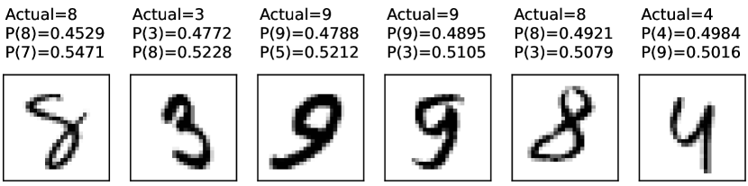
MNIST (Modified National Institute of Standards and Technology database) is a dataset of grayscale images of hand-written digits. Each image consists of a $28\times 28$ grid of pixels, where each pixel is an integer in the range $[0,255]$ specifying its intensity. Some examples are shown in Figure 8.5. There are 60,000 training images and 10,000 test images. MNIST has been used for many perceptual learning case studies.

This was trained with a network with 784 input units (one for each pixel), and one hidden layer containing 512 units with ReLU activation. There are 10 output units, one for each digit, combined with a softmax. It was optimized for categorical cross entropy, and trained for five epochs (each example was used five times, on average, in the training), with a batch size of 128.

After training, the model has a training log loss (base $e$ ) of 0.21, with an accuracy of 98.4% (the mode is the correct label). On the test set the log loss is 0.68, with an accuracy of 97.0%. If trained for more epochs, the fit to the training data gets better, but on the test set, the log loss becomes much worse and accuracy improves to test 97.7% after 15 more epochs. This is run with the default parameters of Keras; different runs might have different errors, and different extreme examples.

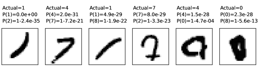
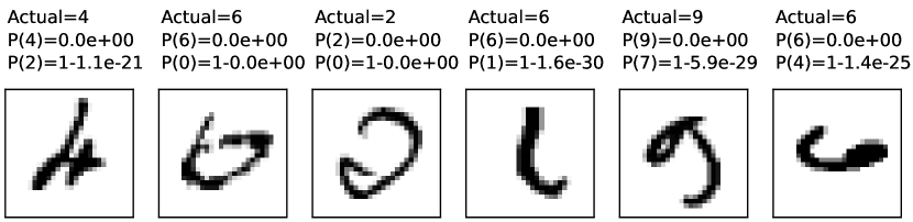
Often, insights can be obtained by looking at the incorrect predictions. Figure 8.5 shows some of the predictions for the images in the training set and the test set. The first two sets of examples are the incorrect predictions that are closest to 0.5; one for the training set and one for the test set. The other two sets of examples are the most extreme incorrect classifications. They have more extreme probabilities than would be justified by the examples.

Artificial Intelligence 3E

8.1 Feedforward Neural Networks

Example 8.1.

8.1.1 Parameter Learning

Example 8.2.

Example 8.3.

Artificial
Intelligence 3E