9 Reasoning with Uncertainty 9.2 Independence 9.4 Probabilistic Inference

9.3 Belief Networks

The notion of conditional independence is used to give a concise representation of many domains. The idea is that, given a random variable $X$ , there may be a few variables that directly affect the $X$ ’s value, in the sense that $X$ is conditionally independent of other variables given these variables. The set of locally affecting variables is called the Markov blanket. This locality is exploited in a belief network.

A belief network is a directed acyclic graph representing conditional dependence among a set of random variables. The random variables are the nodes. The arcs represent direct dependence. The conditional independence implied by a belief network is determined by an ordering of the variables; each variable is independent of its predecessors in the total ordering given a subset of the predecessors called its parents. Independence in the graph is indicated by missing arcs.

To define a belief network on a set of random variables, $\{X_{1},\ldots,X_{n}\}$ , first select a total ordering of the variables, say, $X_{1},\ldots,X_{n}$ . The chain rule (Proposition 9.1.2) shows how to decompose a conjunction into conditional probabilities:

	$\displaystyle P(X_{1}$	$\displaystyle\,{=}\,v_{1}\land X_{2}\,{=}\,v_{2}\land\cdots\land X_{n}\,{=}\,v% _{n})$
		$\displaystyle\mbox{}=\prod_{i=1}^{n}P(X_{i}\,{=}\,v_{i}\mid X_{1}\,{=}\,v_{1}% \land\cdots\land X_{i-1}\,{=}\,v_{i-1}).$

Or, in terms of random variables:

\displaystyle P(X_{1},X_{2},\dots,X_{n})

\displaystyle=\prod_{i=1}^{n}P(X_{i}\mid X_{1},\dots,X_{i-1}).

(9.1)

Define the parents of random variable $X_{i}$ , written $parents(X_{i})$ , to be a minimal set of predecessors of $X_{i}$ in the total ordering such that the other predecessors of $X_{i}$ are conditionally independent of $X_{i}$ given $parents(X_{i})$ . Thus $X_{i}$ probabilistically depends on each of its parents, but is independent of its other predecessors. That is, $parents(X_{i})\subseteq\{X_{1},\ldots,X_{i-1}\}$ such that

P(X_{i}\mid X_{1},\ldots,X_{i-1})=P(X_{i}\mid parents(X_{i})).

This conditional independence characterizes a belief network.

When there are multiple minimal sets of predecessors satisfying this condition, any minimal set may be chosen to be the parents. There can be more than one minimal set only when some of the predecessors are deterministic functions of others.

Putting the chain rule and the definition of parents together gives

\displaystyle P(X_{1},X_{2},\dots,X_{n})

\displaystyle=\prod_{i=1}^{n}P(X_{i}\mid parents(X_{i})).

The probability over all of the variables, $P(X_{1},X_{2},\dots,X_{n})$ , is called the joint probability distribution. A belief network defines a factorization of the joint probability distribution into a product of conditional probabilities.

A belief network, also called a Bayesian network, is an acyclic directed graph (DAG), where the nodes are random variables. There is an arc from each element of $parents(X_{i})$ into $X_{i}$ . Associated with the belief network is a set of conditional probability distributions that specify the conditional probability of each variable given its parents (which includes the prior probabilities of those variables with no parents).

Thus, a belief network consists of

•

a DAG, where each node is labeled by a random variable
•

a domain for each random variable, and
•

a set of conditional probability distributions giving $P(X\mid parents(X))$ for each variable $X$ .

A belief network is acyclic by construction. How the chain rule decomposes a conjunction depends on the ordering of the variables. Different orderings can result in different belief networks. In particular, which variables are eligible to be parents depends on the ordering, as only predecessors in the ordering can be parents. Some of the orderings may result in networks with fewer arcs than other orderings.

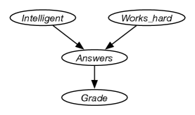
Example 9.11.

Consider the four variables of Example 9.10, with the ordering: $I n t e l l i g e n t$ , $Works\_hard$ , $A n s w e r s$ , $G r a d e$ . Consider the variables in order. $I n t e l l i g e n t$ does not have any predecessors in the ordering, so it has no parents, thus $parents(Intelligent)=\{\}$ . $Works\_hard$ is independent of $I n t e l l i g e n t$ , and so it too has no parents. $A n s w e r s$ depends on both $I n t e l l i g e n t$ and $Works\_hard$ , so

parents(Answers)=\{Intelligent,Works\_hard\}.

$G r a d e$ is independent of $I n t e l l i g e n t$ and $Works\_hard$ given $A n s w e r s$ and so

parents(Grade)=\{Answers\}.

The corresponding belief network is given in Figure 9.2.

This graph defines the decomposition of the joint distribution:

	$\displaystyle P(Inte$	$\displaystyle lligent,Works\_hard,Answers,Grade)$
	$\displaystyle\mbox{}=\mbox{}$	$\displaystyle P(Intelligent)P(Works\_hard)P(Answers\mid Intelligent,Works\_hard)$
		$\displaystyle*P(Grade\mid Answers).$

In the examples below, the domains of the variables are simple, for example the domain of $A n s w e r s$ may be $\{insightful,clear,superficial,vacuous\}$ or it could be the actual text answers.

Refer to caption — Figure 9.2: Belief network for exam answering of Example 9.11

The independence of a belief network, according to the definition of parents, is that each variable is independent of all of the variables that are not descendants of the variable (its non-descendants) given the variable’s parents.

9.3.1 Observations and Queries

A belief network specifies a joint probability distribution from which arbitrary conditional probabilities can be derived. The most common probabilistic inference task – the task required for decision making – is to compute the posterior distribution of a query variable, or variables, given some evidence, where the evidence is a conjunction of assignment of values to some of the variables.

Example 9.12.

Before there are any observations, the distribution over intelligence is $P(Intelligent)$ , which is provided as part of the network. To determine the distribution over grades, $P(Grade)$ , requires inference.

If a grade of $A$ is observed, the posterior distribution of $I n t e l l i g e n t$ is given by

P(Intelligent\mid Grade{\,{=}\,}A).

If it was also observed that $Works\_hard$ is false, the posterior distribution of $I n t e l l i g e n t$ is

P(Intelligent\mid Grade{\,{=}\,}A\land Works\_hard{\,{=}\,}false).

Although $I n t e l l i g e n t$ and $Works\_hard$ are independent given no observations, they are dependent given the grade. This might explain why some people claim they did not work hard to get a good grade; it increases the probability they are intelligent.

9.3.2 Constructing Belief Networks

To represent a domain in a belief network, the designer of a network must consider the following questions.

•
What are the relevant variables? In particular, the designer must consider:
- –
  
  What the agent may observe in the domain. Each feature that may be observed should be a variable, because the agent must be able to condition on all of its observations.
- –
  
  What information the agent is interested in knowing the posterior probability of. Each of these features should be made into a variable that can be queried.
- –
  
  Other hidden variables or latent variables that will not be observed or queried but make the model simpler. These variables either account for dependencies, reduce the size of the specification of the conditional probabilities, or better model how the world is assumed to work.
•

What values should these variables take? This involves considering the level of detail at which the agent should reason to answer the sorts of queries that will be encountered.

For each variable, the designer should specify what it means to take each value in its domain. What must be true in the world for a (non-hidden) variable to have a particular value should satisfy the clarity principle: an omniscient agent should be able to know the value of a variable. It is a good idea to explicitly document the meaning of all variables and their possible values. The only time the designer may not want to do this is for hidden variables whose values the agent will want to learn from data [see Section 10.4.1].
•

What is the relationship between the variables? This should be expressed by adding arcs in the graph to define the parent relation.
•

How does the distribution of a variable depend on its parents? This is expressed in terms of the conditional probability distributions.

Example 9.13.

Suppose you want to use the diagnostic assistant to diagnose whether there is a fire in a building and whether there has been some tampering with equipment based on noisy sensor information and possibly conflicting explanations of what could be going on. The agent receives a report from Sam about whether everyone is leaving the building. Suppose Sam’s report is noisy: Sam sometimes reports leaving when there is no exodus (a false positive), and sometimes does not report when everyone is leaving (a false negative). Suppose that leaving only depends on the fire alarm going off. Either tampering or fire could affect the alarm. Whether there is smoke only depends on whether there is fire.

Suppose you use the following variables in the following order:

•

$T a m p e r i n g$ is true when there is tampering with the alarm.
•

$F i r e$ is true when there is a fire.
•

$A l a r m$ is true when the alarm sounds.
•

$S m o k e$ is true when there is smoke.
•

$L e a v i n g$ is true if there are many people leaving the building at once.
•

$R e p o r t$ is true if Sam reports people leaving. $R e p o r t$ is false if there is no report of leaving.

Assume the following conditional independencies:

•

$F i r e$ is conditionally independent of $T a m p e r i n g$ (given no other information).
•

$A l a r m$ depends on both $F i r e$ and $T a m p e r i n g$ . This is making no independence assumptions about how $A l a r m$ depends on its predecessors given this variable ordering.
•

$S m o k e$ depends only on $F i r e$ and is conditionally independent of $T a m p e r i n g$ and $A l a r m$ given whether there is $F i r e$ .
•

$L e a v i n g$ only depends on $A l a r m$ and not directly on $F i r e$ or $T a m p e r i n g$ or $S m o k e$ . That is, $L e a v i n g$ is conditionally independent of the other variables given $A l a r m$ .
•

$R e p o r t$ only directly depends on $L e a v i n g$ .

The belief network of Figure 9.3 expresses these dependencies.

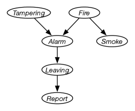
This network represents the factorization

	$\displaystyle P(Tam$	$\displaystyle pering,Fire,Alarm,Smoke,Leaving,Report)$
	$\displaystyle\mbox{}=\mbox{}$	$\displaystyle P(Tampering)P(Fire)P(Alarm\mid Tampering,Fire)$
		$\displaystyleP(Smoke\mid Fire)P(Leaving\mid Alarm)*P(Report\mid Leaving).$

Note that the alarm is not a smoke alarm, which would be affected by the smoke, and not directly by the fire, but rather it is a heat alarm that is directly affected by the fire. This is made explicit in the model in that $A l a r m$ is independent of $S m o k e$ given $F i r e$ .

You also must define the domain of each variable. Assume that the variables are Boolean; that is, they have domain $\{true,false\}$ . We use the lower-case variant of the variable to represent the true value and use negation for the false value. Thus, for example, $Tampering\,{=}\,true$ is written as $t a m p e r i n g$ , and $Tampering\,{=}\,false$ is written as $\neg tampering$ .

The examples that follow assume the following conditional probabilities:

${P(tampering)=0.02}$

${P(fire)=0.01}$

${P(alarm\mid fire\land tampering)=0.5}$

${P(alarm\mid fire\land\neg tampering)=0.99}$

${P(alarm\mid\neg fire\land tampering)=0.85}$

${P(alarm\mid\neg fire\land\neg tampering)=0.0001}$

${P(smoke\mid fire)=0.9}$

${P(smoke\mid\neg fire)=0.01}$

${P(leaving\mid alarm)=0.88}$

${P(leaving\mid\neg alarm)=0.001}$

${P(report\mid leaving)=0.75}$

${P(report\mid\neg leaving)=0.01.}$

Before any evidence arrives, the probability is given by the priors. The following probabilities follow from the model (all of the numbers here are to about three decimal places):

P(tampering)=0.02

P(fire)=0.01

P(report)=0.028

P(smoke)=0.0189.

Observing a report gives the following:

P(tampering\mid report)=0.399

P(fire\mid report)=0.2305

P(smoke\mid report)=0.215.

As expected, the probabilities of both $t a m p e r i n g$ and $f i r e$ are increased by the report. Because the probability of $f i r e$ is increased, so is the probability of $s m o k e$ .

Suppose instead that $s m o k e$ alone was observed:

P(tampering\mid smoke)=0.02

P(fire\mid smoke)=0.476

P(report\mid smoke)=0.320.

Note that the probability of $t a m p e r i n g$ is not affected by observing $s m o k e$ ; however, the probabilities of $r e p o r t$ and $f i r e$ are increased.

Suppose that both $r e p o r t$ and $s m o k e$ were observed:

P(tampering\mid report\land smoke)=0.0284

P(fire\mid report\land smoke)=0.964.

Observing both makes $f i r e$ even more likely. However, in the context of $r e p o r t$ , the presence of $s m o k e$ makes $t a m p e r i n g$ less likely. This is because $r e p o r t$ is explained away by $f i r e$ , which is now more likely.

Suppose instead that $r e p o r t$ , but not $s m o k e$ , was observed:

P(tampering\mid report\land\neg smoke)=0.501

P(fire\mid report\land\neg smoke)=0.0294.

In the context of $r e p o r t$ , $f i r e$ becomes much less likely and so the probability of $t a m p e r i n g$ increases to explain $r e p o r t$ .

This example illustrates how the belief net independence assumption gives commonsense conclusions and also demonstrates how explaining away is a consequence of the independence assumption of a belief network.

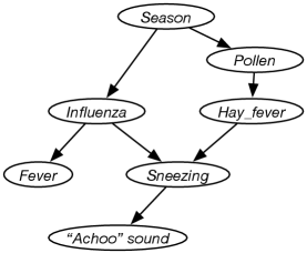
Example 9.14.

Consider the problem of diagnosing why someone is sneezing and perhaps has a fever. Sneezing could be because of influenza or because of hay fever. They are not independent, but are correlated due to the season. Suppose hay fever depends on the season because it depends on the amount of pollen, which in turn depends on the season. The agent does not get to observe sneezing directly, but rather observed just the “Achoo” sound. Suppose fever depends directly on influenza. These dependency considerations lead to the belief network of Figure 9.4.

Example 9.15.

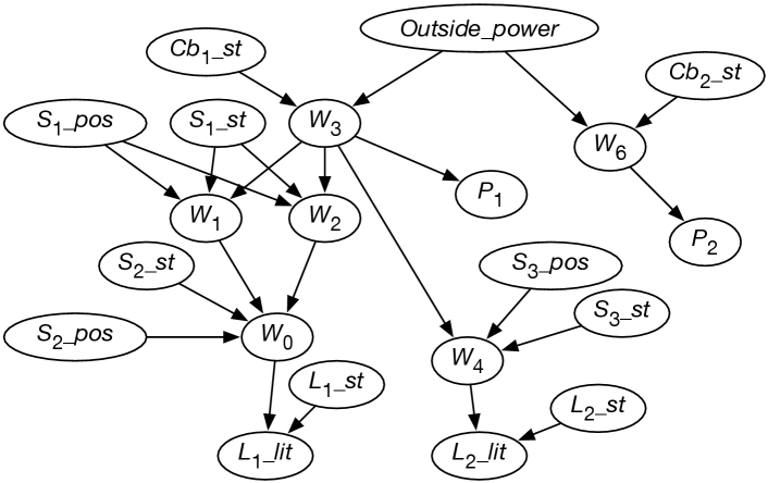
Consider the wiring example of Figure 1.6. Let’s have variables for whether lights are lit, for the switch positions, for whether lights and switches are faulty or not, and for whether there is power in the wires. The variables are defined in Figure 9.5.

Let’s try to order the variables so that each variable has few parents. In this case there seems to be a natural causal order where, for example, the variable for whether a light is lit comes after variables for whether the light is working and whether there is power coming into the light.

Whether light $l_{1}$ is lit depends only on whether there is power in wire $w_{0}$ and whether light $l_{1}$ is working properly. Other variables, such as the position of switch $s_{1}$ , whether light $l_{2}$ is lit, or who is the Queen of Canada, are irrelevant. Thus, the parents of $L_{1}\_lit$ are whether there is power in wire $w_{0}$ (variable $W_{0}$ ), and the status of light $l_{1}$ (variable $L_{1}\_st$ ); see Figure 9.5 for the meaning of the variables.

Consider variable $W_{0}$ , which represents whether there is power in wire $w_{0}$ . If you knew whether there was power in wires $w_{1}$ and $w_{2}$ , and knew the position of switch $s_{2}$ and whether the switch was working properly, the value of the other variables (other than $L_{1}\_lit$ ) would not affect the belief in whether there is power in wire $w_{0}$ . Thus, the parents of $W_{0}$ should be $S_{2}\_Pos$ , $S_{2}\_st$ , $W_{1}$ , and $W_{2}$ .

Figure 9.5 shows the resulting belief network after the independence of each variable has been considered. The belief network also contains the domains of the variables and conditional probabilities of each variable given its parents.

Note the independence assumption embedded in this model. The DAG specifies that the lights, switches, and circuit breakers break independently. To model dependencies among how the switches break, you could add more arcs and perhaps more variables. For example, if some lights do not break independently because they come from the same batch, you could add an extra node modeling the batch, and whether it is a good batch or a bad batch, which is made a parent of the $L_{i}\_st$ variables for each light $L_{i}$ from that batch. When you have evidence that one light is broken, the probability that the batch is bad may increase and thus make it more likely that other lights from that batch are broken. If you are not sure whether the lights are indeed from the same batch, you could add variables representing this, too. The important point is that the belief network provides a specification of independence that lets us model dependencies in a natural and direct manner.

The model implies that there is no possibility of shorts in the wires or that the house is wired differently from the diagram. For example, it implies that $w_{0}$ cannot be shorted to $w_{4}$ so that wire $w_{0}$ gets power from wire $w_{4}$ . You could add extra dependencies that let each possible short be modeled. An alternative is to add an extra node that indicates that the model is appropriate. Arcs from this node would lead to each variable representing power in a wire and to each light. When the model is appropriate, you could use the probabilities of Example 9.15. When the model is inappropriate, you could, for example, specify that each wire and light works at random. When there are weird observations that do not fit in with the original model – they are impossible or extremely unlikely given the model – the probability that the model is inappropriate will increase.

9.3.3 Representing Conditional Probabilities and Factors

A factor is a function of a set of variables; the variables on which it depends are the scope of the factor. Given an assignment of a value to each variable in the scope, the factor evaluates to a number.

A conditional probability is a factor representing $P(Y\mid X_{1},\dots,X_{k})$ , which is a function from the variables $Y,X_{1},\dots,X_{k}$ into nonnegative numbers. It must satisfy the constraints that for each assignment of values to all of $X_{1},\dots,X_{k}$ , the values for $Y$ sum to 1. That is, given values for all of the variables, the function returns a number that satisfies the constraint

\forall x_{1}\dots\forall x_{k}\sum_{y\in domain(Y)}P(Y{\,{=}\,}y\mid X_{1}{\,% {=}\,}x_{1},\dots,X_{k}{\,{=}\,}x_{k})=1.

(9.2)

The following gives a number of ways of representing conditional probabilities, and other factors.

Conditional Probability Tables

A representation for a conditional probability that explicitly stores a value for each assignment to the variables is called a conditional probability table or CPT. This can be done whenever there is a finite set of variables with finite domains. The space used is exponential in the number of variables; the size of the table is the product of the sizes of the domains of the variables in the scope.

One such representation is to use a multidimensional table, storing $P(Y{\,{=}\,}y\mid X_{1}{\,{=}\,}v_{1},\dots,x_{k}{\,{=}\,}v_{k})$ in $p\_y[v_{1}]\dots[v_{k}][y]$ (using Python’s notation for arrays, and exploiting its ambiguity of arrays and dictionaries).

$F i r e$	$T a m p e r i n g$	$P(alarm\mid Fire,Tampering)$
false	false	0.0001
false	true	0.85
true	false	0.99
true	true	0.5

Figure 9.6: Conditional probability of

Alarm{\,{=}\,}true

given

F i r e

and

T a m p e r i n g

Example 9.16.

Figure 9.6 shows the conditional probabilities for $P(alarm\mid Fire,Tampering)$ . The probability for $A l a r m$ being false can be computed from the given probabilities, for example:

P(Alarm{\,{=}\,}false\mid Fire{\,{=}\,}false,Tampering{\,{=}\,}{true})=1-0.85=% 0.15

Given a total ordering of the variables, $[Fire,Tampering,Alarm]$ , the values mapped to the nonnegative integers; false to 0 and true to 1.

$P(Alarm\mid Fire,Tampering)$ of Figure 9.6 can be represented as the Python array

cpt=[[[0.9999,0.0001],[0.15,0.85]],[[0.01,0.99],[0.5,0.5]]].

Given particular values of $Fire{\,{=}\,}f,Tampering{\,{=}\,}t,Alarm{\,{=}\,}a$ , where $f$ , $t$ , and $a$ are each 0 or 1, the value can be found at $cpt[f][t][a]$ . If the domain of a variable is not of the form $\{0,\dots,n-1\}$ , a dictionary can be used. Other languages have different syntaxes.

There are a number of refinements, which use different space-time tradeoffs, including the following.

•

Tables can be implemented as one-dimensional arrays. Given an ordering of the variables (e.g., alphabetical) and an ordering for the values, and using a mapping from the values into nonnegative integers, there is a unique representation using the lexical ordering of each factor as a one-dimensional array that is indexed by natural numbers. This is a space-efficient way to store a table.
•

If the child variable is treated the same as the parent variables, the information is redundant; more numbers are specified than is required. One way to handle this is to store the probability for all-but-one of the values of the child, $Y$ . The probability of the other value can be computed as 1 minus the sum of other values for a set of parents. In particular, if $Y$ is Boolean, you only need to represent the probability for one value, say $Y{\,{=}\,}true$ given the parents; the probability for $Y{\,{=}\,}false$ can be computed from this.
•

It is also possible to store unnormalized probabilities, which are nonnegative numbers that are proportional to the probability. The probability is computed by dividing each value by the sum of the values. This is common when the unnormalized probabilities are counts [see Section 10.2.1].

Decision Trees

The tabular representation of conditional probabilities can be enormous when there are many parents. There is often insufficient evidence – either from data or from experts – to provide all the numbers required. Fortunately, there is often structure in conditional probabilities which can be exploited.

One such structure exploits context-specific independence, where one variable is conditionally independent of another, given particular values for some other variables.

Example 9.17.

Suppose a robot can go outside or get coffee, so $A c t i o n$ has domain $\{go\_out,get\_coffee\}$ . Whether it gets wet (variable $W e t$ ) depends on whether there is rain (variable $R a i n$ ) in the context that it went out or on whether the cup was full (variable $F u l l$ ) if it got coffee. Thus $W e t$ is independent of $R a i n$ given context $Action{\,{=}\,}get\_coffee$ , but is dependent on $R a i n$ given contexts $Action{\,{=}\,}go\_out$ . Also, $W e t$ is independent of $F u l l$ given $Action{\,{=}\,}go\_out$ , but is dependent on $F u l l$ given $Action{\,{=}\,}get\_coffee$ .

A conditional probability table that represents such independencies is shown in Figure 9.7.

$A c t i o n$	$R a i n$	$F u l l$	$P(Wet{\,{=}\,}true\mid Action,Rain,Full)$
go_out	false	false	0.1
go_out	false	true	0.1
go_out	true	false	0.8
go_out	true	true	0.8
get_coffee	false	false	0.3
get_coffee	false	true	0.6
get_coffee	true	false	0.3
get_coffee	true	true	0.6

Figure 9.7: A conditional probability that a robot will get wet

Context-specific independence may be exploited in a representation by not requiring numbers that are not needed. A simple representation for conditional probabilities that models context-specific independence is a decision tree, where the parents in a belief network correspond to the input features that form the splits, and the child corresponds to the target feature. Each leaf of the decision tree contains a probability distribution over the child variable.

Example 9.18.

The conditional probability $P(Wet\mid Action,Rain,Full)$ of Figure 9.7 could be represented as a decision tree, where the number at the leaf is the probability for $Wet{\,{=}\,}true$ :

How to learn a decision tree from data was explored in Section 7.3.1. Context-specific inference can be exploited in probabilistic inference because a factor represented by a decision tree can be evaluated in an assignment when the values down a path in the tree hold; you don’t need to know the value of all parent variables.

Deterministic System with Noisy Inputs

An alternative representation of conditional distributions is in terms of a deterministic system, with probabilistic inputs. The deterministic system can range from a logical formula to a program. The inputs to the system are the parent variables and stochastic inputs. The stochastic inputs – often called noise variables or exogenous variables – can be considered as random variables that are unconditionally independent of each other. There is a deterministic system that defines the non-leaf variables of the belief network, the endogenous variables, as a deterministic function of the exogenous variables and the parents.

When the deterministic system is Clark’s completion of a logic program, it is known as probabilistic logic programming and when the deterministic system is a program, it is known as probabilistic programming. When the deterministic system is specified by a logical formula, the probabilistic inference is known as weighted model counting.

Example 9.19.

The decision tree of Example 9.7 for the conditional distribution of Figure 9.6 can be represented as the logical formula

	$\displaystyle wet\leftrightarrow\mbox{}$	$\displaystyle((go\_out\land rain\land n_{0})$
		$\displaystyle\lor(go\_out\land\neg rain\land n_{1})$
		$\displaystyle\lor(\neg go\_out\land full\land n_{2})$
		$\displaystyle\lor(\neg go\_out\land\neg full\land n_{3}))$

where the $n_{i}$ are independent noise variables, with

\displaystyle P(n_{0})=0.8,~{}P(n_{1})=0.1,~{}P(n_{2})=0.6,~{}P(n_{3})=0.3.

So if, for example, $go\_out$ is true and $r a i n$ is false, then $w e t$ is true whenever $n_{1}$ is true, which occurs with probability 0.1.

This conditional distribution can be represented as a program:

if go_out:
   if rain:
      wet := flip(0.8)
   else:
      wet := flip(0.1)
else:
   if full:
      wet := flip(0.6)
   else:
      wet := flip(0.3)

flip(x) = (random() < x)

where random() returns a random number uniformly in the range [0,1), so flip(x) makes a new independent random variable that is true with probability x. The logical formula gave these random variables names.

Logical formulas allow for much more complicated expressions than presented here. Probabilistic programming allows for the full expressivity of the underlying programming language to express probabilistic models. Typically a single program is used to represent the distribution of all variables, rather than having a separate program for each conditional probability.

Noisy-or

There are many cases where something is true if there is something that makes it true. For example, someone has a symptom if there is a disease that causes that symptom; each of the causes can be probabilistic. In natural language understanding, topics may have words probabilistically associated with them; a word is used if there is a topic that makes that word appear. Each of these examples follows the same pattern, called a noisy-or.

In a noisy-or model of a conditional probability, the child is true if one of the parents is activated and each parent has a probability of activation. So the child is an “or” of the activations of the parents.

If $Y$ has Boolean parents $X_{1},\dots,X_{k}$ , the noisy-or model of probability is defined by $k+1$ parameters $w_{0},\dots,w_{k}$ . $Y$ is defined in terms of a deterministic system with noisy inputs, where

Y\equiv n_{0}\lor(n_{1}\land x_{1})\lor\dots\lor(n_{k}\land x_{k}).

The $n_{i}$ are unconditionally independent noise variables, with $P(n_{i})=w_{i}$ , and $x_{i}$ means $X_{i}{\,{=}\,}true$ .

The same distribution for $P(Y\mid X_{1},X_{2},\dots,X_{k})$ can be defined using $k+1$ Boolean variables $A_{0},A_{1},\dots,A_{k}$ , where for each $i>0$ , $A_{i}$ has $X_{i}$ as its only parent. See Figure 9.8.

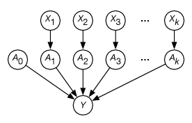
$P(A_{i}{\,{=}\,}true\mid X_{i}{\,{=}\,}true)=w_{i}$ and $P(A_{i}{\,{=}\,}true\mid X_{i}{\,{=}\,}false)=0$ . The variable $A_{0}$ has $P(A_{0}{\,{=}\,}true)=w_{0}$ . The variables $A_{0},\dots,A_{k}$ are the parents of $Y$ . The conditional probability for $Y$ , $P(Y\mid A_{0},A_{1},\dots,A_{k})$ , is 1 if any of the $A_{i}$ are true and 0 if all of the $A_{i}$ are false. Thus, $w_{0}$ is the probability of $Y$ when all of $X_{i}$ are false; the probability of $Y$ increases as more of the $X_{i}$ become true.

Example 9.20.

Suppose the robot could get wet from rain or coffee. There is a probability that it gets wet from rain if it rains, and a probability that it gets wet from coffee if it has coffee, and a probability that it gets wet for other reasons. The robot gets wet if it gets wet from one of the reasons, giving the “or”. You could have $P(wet\_from\_rain\mid rain)=0.3$ , $P(wet\_from\_coffee\mid coffee)=0.2$ , and, for the bias term, $P(wet\_for\_other\_reasons)=0.1$ . The robot is wet if it is wet from rain, wet from coffee, or wet for other reasons.

Log-linear Models and Logistic Regression

In a log-linear model unnormalized probabilities are specified using a product of terms, and probabilities are inferred by normalization. When the terms being multiplied are all positive, a product can be represented as the exponential of a sum. A sum of terms is often a convenient term to work with.

The simplest case is for a Boolean variable. To represent conditional probabilities of a Boolean variable $h$ :

	$\displaystyle P(h\mid e)$	$\displaystyle=\frac{P(h\land e)}{P(e)}$
		$\displaystyle=\frac{P(h\land e)}{P(h\land e)+P(\neg h\land e)}$
		$\displaystyle=\frac{1}{1+P(\neg h\land e)/P(h\land e)}$
		$\displaystyle=\frac{1}{1+\exp(-(\log P(h\land e)/P(\neg h\land e)))}$
		$\displaystyle=sigmoid(\log odds(h\mid e)).$

•

The sigmoid function, $sigmoid(x)=1/(1+\exp(-x))$ , plotted in Figure 7.11, has been used previously in this book for logistic regression and neural networks.
•

The conditional odds (as often used by bookmakers in gambling)

$\displaystyle odds(h\mid e)$ $\displaystyle=\frac{P(h\land e)}{P(\neg h\land e)}$

$\displaystyle=\frac{P(h\mid e)}{P(\neg h\mid e)}$

$\displaystyle=\frac{P(h\mid e)}{1-P(h\mid e)}.$

Decomposing $P(h\land e)$ into $P(e\mid h)*P(h)$ , and analogously for the numerator, gives

$\displaystyle odds(h\mid e)=\frac{P(e\mid h)}{P(e\mid\neg h)}*\frac{P(h)}{P(% \neg h)}$

where $\frac{P(h)}{P(\neg h)}=\frac{P(h)}{1-P(h)}$ is the prior odds and $\frac{P(e\mid h)}{P(e\mid\neg h)}$ is the likelihood ratio. When $P(e\mid h)/P(e\mid\neg h)$ is a product of terms, the log is a sum of terms.

The logistic regression model of a conditional probability $P(Y\mid X_{1},\dots,X_{k})$ is of the form

P(Y{\,{=}\,}true\mid X_{1},\dots,X_{k})=sigmoid\left(\sum_{i}w_{i}*X_{i}\right).

(9.3)

Assume a dummy input $X_{0}$ which is always 1; $w_{0}$ is the bias. This corresponds to a decomposition of the conditional probability, where the likelihood ratio is a product of terms, one for each $X_{i}$ .

Note that $P(Y\mid X_{1}{\,{=}\,}0,\dots,X_{k}{\,{=}\,}0)=sigmoid(w_{0})$ . Thus, $w_{0}$ determines the probability when all of the parents are zero. Each $w_{i}$ specifies a value that should be added as $X_{i}$ changes. $P(Y\mid X_{1}{\,{=}\,}0,\dots,X_{i}{\,{=}\,}1,\dots,X_{k}{\,{=}\,}0)=sigmoid(w% _{0}+w_{i})$ . The logistic regression model makes the independence assumption that the influence of each parent on the child does not depend on the other parents. In particular, it assumes that the odds can be decomposed into a product of terms that each only depend on a single variable. When learning logistic regression models (Section 7.3.2), the training data does not need to obey that independence, but rather the algorithm tries to find a logistic regression model that best predicts the training data (in the sense of having the lowest squared error or log loss).

Example 9.21.

Suppose the probability of $w e t$ given whether there is rain, coffee, kids, or whether the robot has a coat, $P(wet\mid Rain,Coffee,Kids,Coat)$ , is

\displaystyle sigmoid(-1.0+2.0*Rain+1.0*Coffee+0.5*Kids-1.5*Coat).

This implies the following conditional probabilities:

	$\displaystyle P(wet\mid\neg rain\land\neg coffee\land\neg kids\land\neg coat)=% sigmoid(-1.0)=0.27$
	$\displaystyle P(wet\mid rain\land\neg coffee\land\neg kids\land\neg coat)=% sigmoid(1.0)=0.73$
	$\displaystyle P(wet\mid rain\land\neg coffee\land\neg kids\land coat)=sigmoid(% -0.5)=0.38.$

This requires fewer parameters than the $2^{4}=16$ parameters required for a tabular representation, but makes more independence assumptions.

Noisy-or and logistic regression models are similar, but different. Noisy-or is typically used when the causal assumption that a variable is true if it is caused to be true by one of the parents, is appropriate. Logistic regression is used when the various parents add up to influence the child. See the box.

Noisy-or Compared to Logistic Regression

Noisy-or and logistic regression when used for Boolean parents are similar in many ways. They both take a parameter for each parent plus another parameter that is used when all parents are false. Logistic regression cannot represent zero probabilities. Noisy-or cannot represent cases where a parent being true makes the child less probable (although the negation can be a parent).

They can both represent the probability exactly when zero or one parent is true (as long as there are no zero probabilities for logistic regression). They are quite different in how they handle cases when multiple parents are true.

To see the difference, consider representing $P(Y\mid X_{1},X_{2},X_{3},X_{4})$ , using parameters $w_{0},\dots,w_{4}$ . Assume the following probabilities when zero or one parent is true:

\begin{array}[]{llll|l}X_{1}&X_{2}&X_{3}&X_{4}&Prob\\ \hline\cr False&False&False&False&p_{0}{\,{=}\,}0.01\\ True&False&False&False&p_{1}{\,{=}\,}0.05\\ False&True&False&False&p_{2}{\,{=}\,}0.1\\ False&False&True&False&p_{3}{\,{=}\,}0.2\\ False&False&False&True&p_{4}{\,{=}\,}0.2\end{array}

For noisy-or, $w_{0}=p_{0}$ . $1-(1-w_{0})(1-w_{i})=p_{i}$ . Solving for $w_{i}$ gives $w_{i}=1-(1-p_{i})/(1-w_{0})$ .

For logistic regression, $sigmoid(w_{0})=p_{0}$ and $sigmoid(w_{0}+w_{i})=p_{i}$ .

The predictions for $Y{\,{=}\,}true$ for the other assignments to $X$ s are:

\begin{array}[]{llll|l|l}X_{1}&X_{2}&X_{3}&X_{4}&\mbox{Noisy-or}&\mbox{% Logistic Regression}\\ \hline\cr False&False&True&True&0.353535&0.860870\\ False&True&False&True&0.272727&0.733333\\ False&True&True&False&0.272727&0.733333\\ False&True&True&True&0.412305&0.985520\\ True&False&False&True&0.232323&0.565714\\ True&False&True&False&0.232323&0.565714\\ True&False&True&True&0.379655&0.969916\\ True&True&False&False&0.136364&0.366667\\ True&True&False&True&0.302112&0.934764\\ True&True&True&False&0.302112&0.934764\\ True&True&True&True&0.436050&0.997188\end{array}

Logistic regression is much more extreme than noisy-or when multiple $X_{i}$ are true. With noisy-or, each $X_{i}{\,{=}\,}true$ probabilistically forces $Y$ to be true. With logistic regression, each $X_{i}{\,{=}\,}true$ provides independent evidence for $Y$ .

If the probability $p_{0}$ is increased, to say, 0.05, with $p_{1},\dots,p_{4}$ fixed, the probability of $Y{\,{=}\,}true$ given assignments with multiple $X_{i}$ true for noisy-or goes up (as there are more ways $Y$ could be true) and for logistic regression goes down (as each $X_{i}$ true provides less evidence of exceptionality).

One way to extend logistic regression to be able to represent more conditional probabilities is to allow weights for conjunctions of Boolean properties. For example, if Boolean $Y$ has Booleans $X_{1}$ and $X_{2}$ as parents, four weights can be used to define the conditional distribution:

P(y\mid X_{1},X_{2})=sigmoid(w_{0}+w_{1}*X_{1}+w_{2}*X_{2}+w_{3}*X_{1}*X_{2})

where $X_{1}*X_{2}$ is 1 only when both $X_{1}$ and $X_{2}$ are true – the product of variables with domain $\{0,1\}$ corresponds to conjunction. Then

	$\displaystyle w_{0}$	$\displaystyle=logit(P(y\mid X_{1}{\,{=}\,}0,X_{2}{\,{=}\,}0))$
	$\displaystyle w_{1}$	$\displaystyle=logit(P(y\mid X_{1}{\,{=}\,}1,X_{2}{\,{=}\,}0))-w_{0}$
	$\displaystyle w_{2}$	$\displaystyle=logit(P(y\mid X_{1}{\,{=}\,}0,X_{2}{\,{=}\,}1))-w_{0}$
	$\displaystyle w_{3}$	$\displaystyle=logit(P(y\mid X_{1}{\,{=}\,}1,X_{2}{\,{=}\,}1))-w_{0}-w_{1}-w_{2}$

where the logit function is the inverse of the sigmoid.

In general, for $P(Y\mid X_{1},\dots,X_{k})$ there are $2^{k}$ parameters, one for each subset of $\{X_{1},\dots,X_{k}\}$ being conjoined (or multiplied). This is known as the canonical representation. This has the same number of parameters as a conditional probability table, but can be made simpler by not representing the zero weights. Logistic regression is the extreme form where all of the interaction (product) weights are zero. It is common to start with the logistic regression form and add as few interaction terms as needed. This is the representaion of conditioning probabilities for Boolean outputs learned by gradient-boosted trees, with the decision-tree paths representing conjunctions.

A logistic regression model for Boolean variables can be represented using weighted logical formulas, where a weighted logical formula is a pair of a formula and a weight, such that $P(Y{\,{=}\,}true\mid X_{1},\dots,X_{k})$ is proportional to the exponential of the sum of the weights for the formulas for which $Y$ is true, and the $X_{i}$ have their given value. The model of Equation 9.3 can be specified by $(y,w_{0})$ and $(y\land x_{i},w_{i})$ for each $i$ , where $x_{i}$ means $X_{i}{\,{=}\,}true$ . For the canonical representation, more complicated formulas can be used; for example, the case in the previous paragraph is represented by adding the weighted formula $(y\land x_{1}\land x_{2},w_{3})$ to the logistic regression weighted formulas.

The extension of logistic regression to non-binary discrete variables is softmax regression; the softmax of linear functions.

Directed and Undirected Graphical Models

A belief network is a directed model; all of the arcs are directed. The model is defined in terms of conditional probabilities.

An alternative is an undirected model. A factor graph consists of a set of variables and a set of nonnegative factors, each with scope a subset of the variables. There is an arc between each variable and the factors it is in the scope of, similar to a constraint network. It is sometimes written as a Markov random field or Markov network where the factors are implicit: the nodes are the variables, with an edge between any pair of nodes if there is a factor containing both.

The joint probability is defined by

\displaystyle P(X_{1}

\displaystyle\,{=}\,v_{1}\land X_{2}\,{=}\,v_{2}\land\cdots\land X_{n}\,{=}\,v% _{n})\propto\prod_{F}F(X_{F}{\,{=}\,}v_{f})

where $X_{F}$ is the tuple of variables in factor $F$ and $v_{F}$ is the tuple of corresponding values.

The constant of proportionality,

\sum_{X_{1},\dots,X_{n}}\prod_{F}F(X_{F})

is called the partition function. The exact algorithms of Section 9.5 can be used to compute the partition function; those algorithms just assume a set of factors.

Sometimes the factors are defined in terms of weights, so that $F(X_{F_{1}},\dots,X_{F_{k}})=\exp(w_{F}(X_{F_{1}},\dots,X_{F_{k}}))$ . This changes the product above to

\displaystyle P(X_{1}

\displaystyle\,{=}\,v_{1}\land X_{2}\,{=}\,v_{2}\land\cdots\land X_{n}\,{=}\,v% _{n})\propto\exp(\sum_{F}w_{F}(X_{F}{\,{=}\,}v_{f}))

giving a log-linear model, which is useful for learning as the derivative is simpler and the nonnegative constraint happens automatically, although zero probabilities cannot be represented.

Note that a belief network can also be seen as a factor graph, where the factors are defined in terms of conditional probabilities. The directed and undirected models are collectively called graphical models.

A canonical representation is a representation that has a unique form. One problem with undirected models is that there is no canonical representation for a probability distribution. For example, modifying a factor on $X_{i}$ by multiplying $X_{i}{\,{=}\,}v_{i}$ by a constant and modifying another factor on $X_{i}$ by dividing by the same constant gives the same model. This means that the model cannot be learned modularly; each factor depends on the others. A belief network forces a particular factorization that gives a canonical representation for a distribution.

	$\displaystyle odds(h\mid e)$	$\displaystyle=\frac{P(h\land e)}{P(\neg h\land e)}$
		$\displaystyle=\frac{P(h\mid e)}{P(\neg h\mid e)}$
		$\displaystyle=\frac{P(h\mid e)}{1-P(h\mid e)}.$

Artificial Intelligence 3E