10 Learning with Uncertainty 10.3 Unsupervised Learning 10.5 Social Impact

10.4 Learning Belief Networks

A belief network gives a probability distribution over a set of random variables. We cannot always expect an expert to be able to provide an accurate model; often we want to learn a network from data.

Learning a belief network from data has many variants, depending on how much prior information is known and how complete the dataset is. The complexity of learning depends on whether all of the variables are known (or need to be invented), whether the structure is given, and whether all variables are observed, which can vary by example.

The simplest case occurs when a learning agent is given the structure of the model and all variables have been observed. The agent must learn the conditional probabilities, $P(X_{i}\mid parents(X_{i}))$ , for each variable $X_{i}$ . Learning the conditional probabilities is an instance of supervised learning, where $X_{i}$ is the target feature and the parents of $X_{i}$ are the input features. Any of the methods of Chapter 7, Chapter 8, or Section 10.1 can be used to learn the conditional probabilities.

10.4.1 Hidden Variables

The next simplest case is where the model is given, but not all variables are observed. A hidden variable or a latent variable is a variable in a belief network whose value is not observed for any of the examples. That is, there is no column in the data corresponding to that variable.

Refer to caption — Figure 10.9: Deriving probabilities with a hidden variable

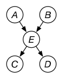
Example 10.11.

Figure 10.9 shows a typical case. Assume that all the variables are binary with domain $\{f,t\}$ . The model contains a hidden variable $E$ that is in the model but not the dataset. The aim is to learn the parameters of the model that includes the hidden variable $E$ . There are 10 parameters to learn.

Note that, if $E$ was not part of the model, the algorithm would have to learn $P(A)$ , $P(B)$ , $P(C\mid AB)$ , $P(D\mid ABC)$ , which has 14 parameters. The reason for introducing hidden variables is, paradoxically, to make the model simpler and, therefore, less prone to overfitting.

The expectation maximization (EM) algorithm for learning belief networks with hidden variables is essentially the same as the EM algorithm for clustering. The E step, depicted in Figure 10.10, involves probabilistic inference for each example to infer the probability distribution of the hidden variable(s) given the observed variables for that example. The M step of inferring the probabilities of the model from the augmented data is the same as in the fully observable case discussed in the previous section, but, in the augmented data, the counts are not necessarily integers.

$A$	$B$	$C$	$D$	$E$	Count
$\vdots$	$\vdots$	$\vdots$	$\vdots$	$\vdots$	$\vdots$
$t$	$f$	$t$	$t$	$t$	0.71
$t$	$f$	$t$	$t$	$f$	0.29
$f$	$f$	$t$	$t$	$f$	4.2
$\vdots$	$\vdots$	$\vdots$	$\vdots$	$\vdots$	$\vdots$
$f$	$t$	$t$	$t$	$f$	2.3

E-step

\longleftarrow

M-step

\longrightarrow

P(A)

P(B)

P(E\mid A,B)

P(C\mid E)

P(D\mid E)

Figure 10.10: EM algorithm for belief networks with hidden variables;

E

is a hidden variable. The E-step computes

P(E\mid A,B,C,D)

for each example, and the M-step learns probabilities from complete data

10.4.2 Missing Data

Data can be incomplete in ways other than having an unobserved variable. A dataset could simply be missing the values of some variables for some of the examples. When some of the values of the variables are missing, one must be very careful in using the dataset because the missing data may be correlated with the phenomenon of interest.

A simple case is when only categorical variables with no parents that are not themselves queried have missing values. A probability distribution from which other variables can be queried can be modeled by adding an extra value “missing” to the domain of the variables with missing values. This can also be modeled by having a 0/1 indicator variable for each value in the domain of the variable, where all of the indicator variables are 0 if the value is missing.

Example 10.12.

Consider a case where someone volunteers information about themself. If someone has a sibling, they are likely to volunteer that; if they do not have a sibling, it is unusual for them to state that. Similarly, if someone doesn’t have anxiety, they are unlikely to mention anxiety, but might mention that they are not anxious. There are too many ailments and other conditions that humans have for them to mention the ones they don’t have. Suppose there is a model of when someone fears isolation ( $f$ ) that depends on whether they have a sibling ( $S$ ) and whether they have anxiety ( $A$ ). A logistic regression model could be

	$\displaystyle P(f)=sigmoid($	$\displaystyle w_{0}+w_{1}(S{\,{=}\,}true)+w_{2}(S{\,{=}\,}false)$
		$\displaystyle+w_{3}(A{\,{=}\,}true)+w_{4}(A{\,{=}\,}false))$

where $S{\,{=}\,}true$ has value 1 when $S$ is reported to be true, and $S{\,{=}\,}false$ has value 1 when $S$ is reported to be false, and both have value 0 when the value is missing. The learned bias, $w_{0}$ , is the value used when both $S$ and $A$ are missing.

In general, missing data cannot be ignored, as in the following example.

Example 10.13.

Suppose there is a drug that is a (claimed) treatment for a disease that does not actually affect the disease or its symptoms. All it does is make sick people sicker. Suppose patients were randomly assigned to the treatment, but the sickest people dropped out of the study, because they became too sick to participate. The sick people who took the treatment were sicker and so would drop out at a faster rate than the sick people who did not take the treatment. Thus, if the patients with missing data are ignored, it looks like the treatment works; there are fewer sick people among the people who took the treatment and remained in the study!

Handling missing data requires more than a probabilistic model that models correlation. It requires a causal model of how the data is missing; see Section 11.2.

10.4.3 Structure Learning

Suppose a learning agent has complete data and no hidden variables, but is not given the structure of the belief network. This is the setting for structure learning of belief networks.

There are two main approaches to structure learning:

•

The first is to use the definition of a belief network in terms of conditional independence. Given a total ordering of variables, the parents of a variable $X$ are defined to be a subset of the predecessors of $X$ in the total ordering that render the other predecessors independent of $X$ . Using the definition directly has two main challenges: the first is to determine the best total ordering; the second is to find a way to measure independence. It is difficult to determine conditional independence when there is limited data.
•

The second method is to have a score for networks, for example, using the MAP model, which takes into account fit to the data and model complexity. Given such a measure, it is feasible to search for the structure that minimizes this error.

This section presents the second method, often called a search and score method.

Assume that the data is a set $E$ of examples, where each example has a value for each variable. The aim of the search and score method is to choose a model $m$ that maximizes

P(m\mid E)\propto P(E\mid m)*P(m).

The likelihood, $P(E\mid m)$ , is the product of the probability of each example. Using the product decomposition, the product of each example given the model is the product of the probability of each variable given its parents in the model. Thus

	$\displaystyle P(E\mid m)*P(m)$	$\displaystyle\mbox{}=\left(\prod_{e\in E}P(e\mid m)\right)*P(m)$
		$\displaystyle\mbox{}=\left(\prod_{e\in E}\prod_{X_{i}}P_{m}^{e}(X_{i}\mid par(% X_{i},m))\right)*P(m)$

where $par(X_{i},m)$ denotes the parents of $X_{i}$ in the model $m$ , and $P_{m}^{e}(\cdot)$ denotes the probability of example $e$ as specified in the model $m$ .

This is maximized when its logarithm is maximized. When taking logarithms, products become sums:

\displaystyle\log P(E\mid m)+\log P(m)=\left(\sum_{e\in E}\sum_{X_{i}}\log P_{% m}^{e}(X_{i}\mid par(X_{i},m))\right)+\log P(m).

To make this approach feasible, assume that the prior probability of the model decomposes into components for each variable. That is, we assume the probability of the model decomposes into a product of probabilities of local models for each variable. Let $m(X_{i})$ be the local model for variable $X_{i}$ .

Thus, we want to maximize

	$\displaystyle{\left(\sum_{e\in E}\sum_{X_{i}}\log P_{m}^{e}(X_{i}\mid par(X_{i% },m))\right)+\sum_{X_{i}}\log P(m(X_{i}))}$
	$\displaystyle=\sum_{X_{i}}\left(\sum_{e\in E}\log P_{m}^{e}(X_{i}\mid par(X_{i% },m))\right)+\sum_{X_{i}}\log P(m(X_{i}))$
	$\displaystyle=\sum_{X_{i}}\left(\sum_{e\in E}\log P_{m}^{e}(X_{i}\mid par(X_{i% },m))+\log P(m(X_{i}))\right).$

Each variable could be optimized separately, except for the requirement that a belief network is acyclic. However, if you had a total ordering of the variables, there is an independent supervised learning problem to predict the probability of each variable given the predecessors in the total ordering. To approximate $\log P(m(X_{i}))$ , the BIC score can be used. To find a good total ordering of the variables, a learning agent could search over total orderings, using search techniques such as local search or branch-and-bound search.

10.4.4 General Case of Belief Network Learning

The general case has unknown structure, hidden variables, and missing data; we may not even know which variables should be part of the model. Two main problems arise. The first is the problem of missing data discussed earlier. The second is computational; although there may be a well-defined search space, it is prohibitively large to try all combinations of variable ordering and hidden variables. If one only considers hidden variables that simplify the model (as is reasonable), the search space is finite, but enormous.

One can either select the best model (e.g., the model with the highest posterior probability) or average over all models. Averaging over all models gives better predictions, but it is difficult to explain to a person who may have to understand or justify the model.

Artificial Intelligence 3E