Artificial
Intelligence 3E
foundations of computational agents
10.3 Unsupervised Learning
This chapter has so far considered supervised learning, where target features are observed in the training data. In unsupervised learning, the target features are not given in the training examples.
One general method for unsupervised learning is clustering, which partitions the examples into clusters. Each cluster predicts feature values for the examples in the cluster. The best clustering is the one that minimizes the prediction error, such as squared error or log loss.
Often the term class is used as a semantically meaningful term, but while you might want the clusters to be semantically meaningful, they are not always.
Example 10.8.
A diagnostic assistant may want to group treatments into groups that predict the desirable and undesirable effects of the treatment. The assistant may not want to give a patient a drug because similar drugs may have had disastrous effects on similar patients.
A tutoring agent may want to cluster students’ learning behavior so that strategies that work for one member of a cluster may work for other members.
In hard clustering, each example is placed definitively in a cluster. The cluster is then used to predict the feature values of the example. The alternative to hard clustering is soft clustering, in which each example has a probability distribution over clusters. The prediction of the values for the features of an example is the weighted average of the predictions of the clusters the example is in, weighted by the probability of the example being in the cluster. Soft clustering is described in Section 10.3.2.
10.3.1 k-Means
The k-means algorithm is used for hard clustering. The training examples, , and the number of clusters, , are given as input. It requires the value of each feature to be a (real) number, so that differences in values make sense.
The algorithm constructs clusters, a prediction of a value for each feature for each cluster, and an assignment of examples to clusters.
Suppose the input features, , are observed for each example. Let be the value of input feature for example . Associate a cluster with each integer .
The -means algorithm constructs
-
•
a function that maps each example to a cluster (if , example is said to be in cluster )
-
•
a function that returns the predicted value of each element of cluster on feature .
Example is thus predicted to have value for feature .
The aim is to find the functions and that minimize the sum of squared loss:
To minimize the squared loss, the prediction of a cluster should be the mean of the prediction of the examples in the cluster; see Figure 7.5. Finding an optimal clustering is NP-hard. When there are only a few examples, it is possible to enumerate the assignments of examples to clusters. For more than a few examples, there are too many partitions of the examples into clusters for exhaustive search to be feasible.
The -means algorithm iteratively improves the squared loss. Initially, it randomly assigns the examples to clusters. Then it carries out the following two steps:
-
•
For each cluster and feature , make be the mean value of for each example in cluster :
where the denominator is the number of examples in cluster .
-
•
Reassign each example to a cluster: assign each example to a cluster that minimizes
These two steps are repeated until the second step does not change the assignment of any example.
An algorithm that implements -means is shown in Figure 10.4. It constructs sufficient statistics to compute the mean of each cluster for each feature, namely
-
•
is the number of examples in cluster
-
•
is the sum of the value for for examples in cluster .
These are sufficient statistics because they contain all of the information from the data necessary to compute and . The current values of and are used to determine the next values (in and ).
The random initialization could be assigning each example to a cluster at random, selecting points at random to be representative of the clusters, or assigning some, but not all, of the examples to construct the initial sufficient statistics. The latter two methods may be more useful if the dataset is large, as they avoid a pass through the whole dataset for initialization.
An assignment of examples to clusters is stable if an iteration of -means does not change the assignment. Stability requires that in the definition of gives a consistent value for each example in cases where more than one cluster is minimal. This algorithm has reached a stable assignment when each example is assigned to the same cluster in one iteration as in the previous iteration. When this happens, and do not change, and so the Boolean variable becomes .
This algorithm will eventually converge to a stable local minimum. This is easy to see because the sum-of-squares error keeps reducing and there are only a finite number of reassignments. This algorithm often converges in a few iterations.
Example 10.9.
Suppose an agent has observed the pairs
, , , , , , , , , , , , , .
These data points are plotted in Figure 10.5(a). The agent wants to cluster the data points into two clusters ().
In Figure 10.5(b), the points are randomly assigned into the clusters; one cluster is depicted as and the other as . The mean of the points marked with is , shown with . The mean of the points marked with is , shown with .
In Figure 10.5(c), the points are reassigned according to the closer of the two means. After this reassignment, the mean of the points marked with is then . The mean of the points marked with is .
In Figure 10.5(d), the points are reassigned to the closest mean. This assignment is stable in that no further reassignment will change the assignment of the examples.
A different initial assignment to the points can give different clustering. One clustering that arises in this dataset is for the lower points (those with a -value less than 3) to be in one cluster, and for the other points to be in another cluster.
Running the algorithm with three clusters () typically separates the data into the top-right cluster, the left-center cluster, and the lower cluster. However, there are other possible stable assignments that could be reached, such as having the top three points in two different clusters, and the other points in another cluster.
Some stable assignments may be better, in terms of sum-of-squares error, than other stable assignments. To find the best assignment, it is often useful to try multiple starting configurations, using a random restart and selecting a stable assignment with the lowest sum-of-squares error. Note that any permutation of the labels of a stable assignment is also a stable assignment, so there are invariably multiple local and global minima.
One problem with the -means algorithm is that it is sensitive to the relative scale of the dimensions. For example, if one feature is in centimeters, another feature is , and another is a binary () feature, the different values need to be scaled so that they can be compared. How they are scaled relative to each other affects the clusters found. It is common to scale the dimensions to between 0 and 1 or with a mean of 0 and a variance of 1, but this assumes that all dimensions are relevant and independent of each other.
Finding an appropriate number of clusters is a classic problem in trading off model complexity and fit to data. One solution is to use the Bayesian information criteria (BIC) score, similar to its use in decision trees where the number of clusters is used instead of the number of leaves. While it is possible to construct clusters from clusters, the optimal division into three clusters, for example, may be quite different from the optimal division into two clusters.
10.3.2 Expectation Maximization for Soft Clustering
A hidden variable or latent variable is a probabilistic variable that is not observed in a dataset. A Bayes classifier can be the basis for unsupervised learning by making the class a hidden variable.
The expectation maximization (EM) algorithm can be used to learn probabilistic models with hidden variables. Combined with a naive Bayes classifier, it does soft clustering, similar to the -means algorithm, but where examples are probabilistically in clusters.
As in the -means algorithm, the training examples and the number of clusters, , are given as input.
| Data | Model | ➪ | Probabilities |
|---|---|---|---|
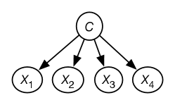 |
Given the data, a naive Bayes model is constructed where there is a variable for each feature in the data and a hidden variable for the class. The class variable is the only parent of the other features. This is shown in Figure 10.6. The class variable has domain , where is the number of classes. The probabilities needed for this model are the probability of the class and the probability of each feature given . The aim of the EM algorithm is to learn probabilities that best fit the data.
The EM algorithm conceptually augments the data with a class feature, , and a count column. Each original example gets mapped into augmented examples, one for each class. The counts for these examples are assigned so that they sum to 1.
For four features and three classes, the example is mapped into the three tuples, shown in the table on the left of Figure 10.7. EM works by iteratively determining the count from the model, and the model from the count.
|
|
|
The EM algorithm repeats the following two steps:
-
•
E step. Update the augmented counts based on the probability distribution. For each example in the original data, the count associated with in the augmented data is updated to
This step involves probabilistic inference. If multiple examples have the same values for the input features, they can be treated together, with the probabilities multiplied by the number of examples. This is an expectation step because it computes the expected values.
-
•
M step. Infer the probabilities for the model from the augmented data. Because the augmented data has values associated with all the variables, this is the same problem as learning probabilities from data in a naive Bayes classifier. This is a maximization step because it computes the maximum likelihood estimate or the maximum a posteriori probability (MAP) estimate of the probability.
The EM algorithm starts with random probabilities or random counts. EM will converge to a local maximum of the likelihood of the data.
This algorithm returns a probabilistic model, which is used to classify an existing or new example. An example is classified using
The algorithm does not need to store the augmented data, but can maintain a set of sufficient statistics, which is enough information to compute the required probabilities. Assuming categorical features, sufficient statistics for this algorithm are
-
•
, the class count, a -valued array such that is the sum of the counts of the examples in the augmented data with
-
•
, the feature count, a three-dimensional array; for from 1 to , for each value in , and for each class , is the sum of the counts of the augmented examples with and .
In each iteration, it sweeps through the data once to compute the sufficient statistics. The sufficient statistics from the previous iteration are used to infer the new sufficient statistics for the next iteration.
The probabilities required of the model can be computed from and :
where is the number of examples in the original dataset (which is the same as the sum of the counts in the augmented dataset).
The algorithm of Figure 10.8 computes the sufficient statistics. Evaluating in line 17 relies on the counts in and . This algorithm has glossed over how to initialize the counts. One way is for to return a random distribution for the first iteration, so the counts come from the data. Alternatively, the counts can be assigned randomly before seeing any data. See Exercise 10.7.
The algorithm will eventually converge when and do not change significantly in an iteration. The threshold for the approximately equal in line 21 can be tuned to trade off learning time and accuracy. An alternative is to run the algorithms for a fixed number of iterations.
Example 10.10.
Consider Figure 10.7.
When example is encountered in the dataset, the algorithm computes
for each class and normalizes the results. Suppose the value computed for class is 0.4, class 2 is 0.1, and class 3 is 0.5 (as in the augmented data in Figure 10.7). Then is incremented by , is incremented by , etc. Values , , etc. are each incremented by . Next, , are each incremented by , etc.
Notice the similarity with the -means algorithm. The E step (probabilistically) assigns examples to classes, and the M step determines what the classes predict.
As long as , EM, like -means, virtually always has multiple local and global maxima. In particular, any permutation of the class labels will give the same probabilities. To try to find a global maximum, multiple restarts can be tried, and a model with the lowest log-likelihood returned.
Artificial Intelligence: Foundations of Computational Agents, Poole
& Mackworth
Copyright © 2023, David L. Poole and Alan K. Mackworth. 
This work is licensed under a Creative Commons Attribution-NonCommercial-NoDerivatives 4.0 International License.