Artificial
Intelligence 3E
foundations of computational agents
3.6 Informed (Heuristic) Search
The search methods in the preceding section are uninformed in that they do not take the goal into account until they expand a path that leads to a goal node. Heuristic information about which nodes are most promising can guide the search by changing which node is selected in line 13 of the generic search algorithm in Figure 3.5.
A heuristic function takes a node and returns a non-negative real number that is an estimate of the cost of the least-cost path from node to a goal node. The function is an admissible heuristic if is always less than or equal to the actual cost of a lowest-cost path from node to a goal.
There is nothing magical about a heuristic function. It must use only information that can be readily obtained about a node. Typically there is a trade-off between the amount of work it takes to compute a heuristic value for a node and the accuracy of the heuristic value.
A standard way to derive a heuristic function is to solve a simpler problem and to use the cost to the goal in the simplified problem as the heuristic function of the original problem [see Section 3.6.3].
Example 3.14.
For the graph of Figure 3.3, if the cost is the distance, the straight-line distance between the node and its closest goal can be used as the heuristic function.
The examples that follow assume the following heuristic function for the goal :
This function is an admissible heuristic because the value is less than or equal to the exact cost of a lowest-cost path from the node to a goal. It is the exact cost for node . It is very much an underestimate of the cost to the goal for node , which seems to be close, but there is only a long route to the goal. It is very misleading for , which also seems close to the goal, but it has no path to the goal.
The function can be extended to be applicable to paths by making the heuristic value of a path equal to the heuristic value of the node at the end of the path. That is:
A simple use of a heuristic function in depth-first search is to order the neighbors that are added to the stack representing the frontier. The neighbors can be added to the frontier so that the best neighbor is selected first. This is known as heuristic depth-first search. This search selects the locally best path, but it explores all paths from the selected path before it selects another path. Although it is often used, it suffers from the problems of depth-first search, is not guaranteed to find a solution, and may not find an optimal solution.
Another way to use a heuristic function is to always select a path on the frontier with the lowest heuristic value. This is called greedy best-first search. This method is not guaranteed to find a solution when there is one.
Example 3.15.
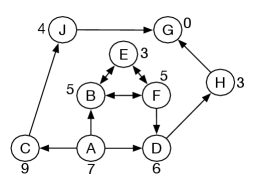
Consider the graph shown in Figure 3.12, where the heuristic value to is shown for each node. The arc costs are ignored and so are not shown. The aim is to find the shortest path from to . A heuristic depth-first search and greedy best-first search will cycle forever in the nodes , , and will never terminate. Even if one could detect the cycles, it is possible to have a similar graph with infinitely many nodes connected, all with a heuristic value less that 6, which would still be problematic for heuristic depth-first search and greedy best-first search.
3.6.1 Search
search finds a least-cost path and can exploit heuristic information to improve the search. It uses both path cost, as in lowest-cost-first, and a heuristic function, as in greedy best-first search, in its selection of which path to expand. For each path on the frontier, uses an estimate of the total path cost from the start node to a goal node that follows then goes to a goal. It uses , the cost of the path found, as well as the heuristic function , the estimated path cost from the end of to the goal.
For any path on the frontier, define . This is an estimate of the total path cost to follow path then go to a goal node. If is the node at the end of path , this can be depicted as
If is an admissible heuristic and so never overestimates the cost from node to a goal node, then does not overestimate the path cost of going from the start node to a goal node via .
is implemented using the generic search algorithm, treating the frontier as a priority queue ordered by .
Example 3.16.
Consider using search for the graph of Figure 3.3 using the heuristic function of Example 3.14, shown in Figure 3.13.
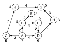
In this example, the paths on the frontier are shown using the final node of the path, subscripted with the -value of the path. The frontier is initially , because and the cost of the path is zero. It is replaced by its neighbors, forming the frontier
The first element of the frontier has . Because it has the lowest -value, is expanded, forming the frontier
The path to is selected, but has no neighbors, so the path is removed. Then there are two paths with the same -value of 10. The algorithm does not specify which is selected. Suppose it expands the path to the node with the smallest heuristic value (see Exercise 3.6), which is the path to . The resulting frontier is
Then the path to is expanded, forming
Next the path to is expanded, forming the frontier
The path is returned, as the shortest path to a goal with a cost of 11.
Notice how the path to was never selected. There could have been a huge network leading from which would never have been explored, as recognized that any such path could not be optimal.
Example 3.17.
Consider Figure 3.12 with cycles. This was problematic for greedy best-first search that ignores path costs. Although initially searches through , , and , eventually the cost of the path becomes so large that it selects the optimal path via and .
A search algorithm is admissible if, whenever a solution exists, it returns an optimal solution. To guarantee admissibility, some conditions on the graph and the heuristic must hold. The following theorem gives sufficient conditions for to be admissible.
Proposition 3.1.
( admissibility) If there is a solution, using heuristic function always returns an optimal solution if:
-
•
the branching factor is bounded above by some number (each node has or fewer neighbors)
-
•
all arc costs are greater than some
-
•
is an admissible heuristic, which means that is less than or equal to the actual cost of the lowest-cost path from node to a goal node.
Proof.
Part A: A solution will be found. If the arc costs are all greater than some , the costs are bounded above zero. If this holds and with a finite branching factor, eventually, for all paths in the frontier, will exceed any finite number and, thus, will exceed a solution cost if one exists (with each path having no greater than arcs, where is the cost of an optimal solution). Because the branching factor is finite, only a finite number of paths must be expanded before the search could get to this point, but the search would have found a solution by then. Bounding the arc costs above zero is a sufficient condition for to avoid suffering from Zeno’s paradox, as described for lowest-cost-first search.
Part B: The first path to a goal selected is an optimal path. is admissible implies the -value of a node on an optimal solution path is less than or equal to the cost of an optimal solution, which, by the definition of optimal, is less than the cost for any non-optimal solution. The -value of a solution is equal to the cost of the solution if the heuristic is admissible. Because an element with minimum -value is selected at each step, a non-optimal solution can never be selected while there is a path on the frontier that leads to an optimal solution. So, before it can select a non-optimal solution, will have to pick all of the nodes on an optimal path, including an optimal solution. ∎
It should be noted that the admissibility of does not ensure that every intermediate node selected from the frontier is on an optimal path from the start node to a goal node. Admissibility ensures that the first solution found will be optimal even in graphs with cycles. It does not ensure that the algorithm will not change its mind about which partial path is the best while it is searching.
To see how the heuristic function improves the efficiency of , suppose is the cost of a least-cost path from the start node to a goal node. , with an admissible heuristic, expands all paths from the start node in the set
and some of the paths in the set
Increasing while keeping it admissible can help reduce the size of the first of these sets. Admissibility means that if a path is in the first set, then so are all of the initial parts of , which means they will all be expanded. If the second set is large, there can be a great variability in the space and time of . The space and time can be sensitive to the tie-breaking mechanism for selecting a path from those with the same -value. It could, for example, select a path with minimal -value or use a first-in, last-out protocol (the same as a depth-first search) for these paths; see Exercise 3.6.
3.6.2 Branch and Bound
Depth-first branch-and-bound search is a way to combine the space saving of depth-first search with heuristic information for finding optimal paths. It is particularly applicable when there are many paths to a goal. As in search, the heuristic function is non-negative and less than or equal to the cost of a lowest-cost path from to a goal node.
The idea of a branch-and-bound search is to maintain the lowest-cost path to a goal found so far, and its cost. Suppose this cost is . If the search encounters a path such that , path can be pruned. If a non-pruned path to a goal is found, it must be better than the previous best path. This new solution is remembered and is reduced to the cost of this new solution. The searcher then proceeds to search for a better solution.
Once it has found one solution, branch-and-bound search generates a sequence of ever-improving solutions. The final solution found is the optimal solution.
Branch-and-bound search is typically used with depth-first search, where the space saving of the depth-first search can be achieved. It can be implemented similarly to depth-bounded search, but where the bound is in terms of path cost and reduces as shorter paths are found. The algorithm remembers the lowest-cost path found and returns this path when the search finishes.
The algorithm is shown in Figure 3.14. The internal procedure , for cost-bounded search, uses the global variables to provide information to the main procedure.
Initially, can be set to infinity, but it is often useful to set it to an overestimate, , of the path cost of an optimal solution. This algorithm will return an optimal solution – a lowest-cost path from the start node to a goal node – if there is a solution with cost less than the initial bound .
If the initial bound is slightly above the cost of a lowest-cost path, this algorithm can find an optimal path expanding no more arcs than search. However, it is rare to know the cost of a lowest-cost path. In general, once it has found an optimal path to the goal, it only explores paths whose -value is lower than the optimal path. These are exactly the paths that explores to find one solution.
If it returns when , there are no solutions. If it returns when is some finite value, it means no solution exists with cost less than . This algorithm can be combined with iterative deepening to increase the bound until either a solution is found or it can show there is no solution, using a method similar to the use of in Figure 3.11. See Exercise 3.11.
Example 3.18.
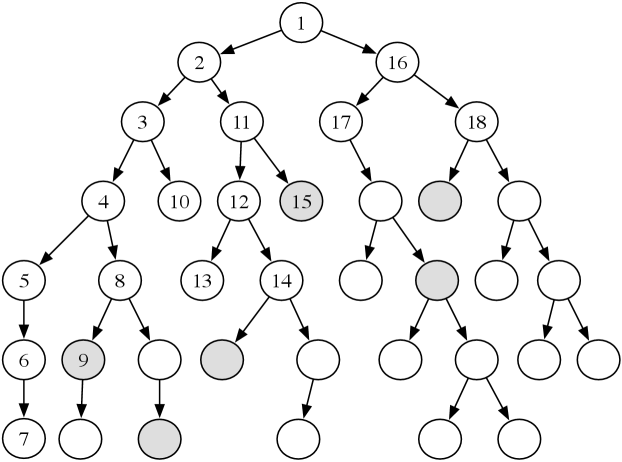
Consider the tree-shaped graph in Figure 3.15. The goal nodes are shaded. Suppose that each arc has cost 1, and there is no heuristic information (i.e., for each node ). In the algorithm, suppose and the depth-first search always selects the leftmost child first. This figure shows the order in which the nodes are checked to determine if they are a goal node. The nodes that are not numbered are not checked for being a goal node.
The subtree under the node numbered “5” does not have a goal and is explored fully (or up to depth if it had a finite value). The ninth node checked is a goal node. It has a path cost of 5, and so the bound is set to 5. From then on, only paths with a cost of less than 5 are checked for being a solution. The fifteenth node checked is also a goal. It has a path cost of 3, and so the bound is reduced to 3. There are no other goal nodes found, and so the path to the node labeled 15 is returned. It is an optimal path. Another optimal path is pruned; the algorithm never checks the children of the node labeled 18.
If there were heuristic information, it could also be used to prune parts of the search space, as in search.
3.6.3 Designing a Heuristic Function
An admissible heuristic is a non-negative function of nodes, where is never greater than the actual cost of the shortest path from node to a goal. The standard way to construct a heuristic function is to find a solution to a simpler problem, one with fewer states or fewer constraints. A problem with fewer constraints is often easier to solve (and sometimes trivial to solve). An optimal solution to the simpler problem cannot have a higher cost than an optimal solution to the full problem because any solution to the full problem is a solution to the simpler problem.
In many spatial problems where the cost is distance and the solution is constrained to go via predefined arcs (e.g., road segments), the straight-line Euclidean distance between two nodes is an admissible heuristic because it is the solution to the simpler problem where the agent is not constrained to go via the arcs.
For many problems one can design a better heuristic function, as in the following examples.
Example 3.19.
Consider the delivery robot of Example 3.4, where the state space includes the parcels to be delivered. Suppose the cost function is the total distance traveled by the robot to deliver all the parcels. If the robot could carry multiple parcels, one possible heuristic function is the maximum of (a) and (b):
-
(a)
the maximum delivery distance for any of the parcels that are not at their destination and not being carried, where the delivery distance of a parcel is the distance to that parcel’s location plus the distance from that parcel’s location to its destination
-
(b)
the distance to the furthest destination for the parcels being carried.
This is not an overestimate because it is a solution to the simpler problem which is to ignore that it cannot travel though walls, and to ignore all but the most difficult parcel. Note that a maximum is appropriate here because the agent has to both deliver the parcels it is carrying and go to the parcels it is not carrying and deliver them to their destinations.
If the robot could only carry one parcel, one possible heuristic function is the sum of the distances that the parcels must be carried plus the distance to the closest parcel. Note that the reference to the closest parcel does not imply that the robot will deliver the closest parcel first, but is needed to guarantee that the heuristic is admissible.
Example 3.20.
In the route planning of Example 3.1, when minimizing time, a heuristic could use the straight-line distance from the current location to the goal divided by the maximum speed – assuming the user could drive straight to the destination at top speed.
A more sophisticated heuristic may take into account the different maximum speeds on highways and local roads. One admissible heuristic is the minimum of (a) and (b):
-
(a)
the estimated minimum time required to drive straight to the destination on slower local roads
-
(b)
the minimum time required to drive to a highway on slow roads, then drive on highways to a location close to the destination, then drive on local roads to the destination.
The minimum is appropriate here because the agent can go via highways or local roads, whichever is quicker.
In the above examples, determining the heuristic did not involve search. Once the problem is simplified, it could be solved using search, which should be simpler than the original problem. The simpler search problem typically needs to be solved multiple times, even perhaps for all nodes. It is often useful to cache these results into a pattern database that maps the nodes of the simpler problem into the heuristic value. In the simpler abstract problem, there are often fewer nodes, with multiple original nodes mapped into a single node in the simplified graph, which can make storing the heuristic value for each of these nodes feasible.
Artificial Intelligence: Foundations of Computational Agents, Poole
& Mackworth
Copyright © 2023, David L. Poole and Alan K. Mackworth. 
This work is licensed under a Creative Commons Attribution-NonCommercial-NoDerivatives 4.0 International License.