9 Reasoning with Uncertainty 9.4 Probabilistic Inference 9.6 Sequential Probability Models

9.5 Exact Probabilistic Inference

The task of probabilistic inference is to compute the probability of a query variable $Q$ given evidence $e$ , where $e$ is a conjunction of assignments of values to some of the variables; that is, to compute $P(Q\mid e)$ . This is the task that is needed for decision making.

Given evidence $e$ , and query variable or variables $Q$ , the problem of computing the posterior distribution on $Q$ can be reduced to the problem of computing the probability of conjunctions, using the definition of conditioning:

	$\displaystyle P(Q\mid e)$	$\displaystyle\mbox{}=\frac{P(Q\land e)}{P(e)}$
		$\displaystyle\mbox{}=\frac{P(Q\land e)}{\displaystyle\sum_{Q}P(Q\land e)}$		(9.4)

where $\displaystyle\sum_{Q}$ means summing over all of the values of $Q$ , which is called marginalizing $Q$ and $\displaystyle\sum_{Q}P(Q\land e)$ is an abbreviation for $\displaystyle\sum_{v\in domain(Q)}P(Q{\,{=}\,}v\land e)$ , where $Q{\,{=}\,}v$ is the proposition that is true when $Q$ has value $v$ .

To compute the probability of a product, first introduce all of the other variables. With all of the variables, the definition of a belief network is used to decompose the resulting joint probability into a product of factors.

Suppose $\{X_{1},\ldots,X_{n}\}$ is the set of all variables in the belief network and the evidence $e$ is $Y_{1}{\,{=}\,}v_{1},\ldots,Y_{j}{\,{=}\,}v_{j}$ , where $\{Y_{1},\dots,Y_{j}\}\subseteq\{X_{1},\ldots,X_{n}\}$ .

Suppose $Z_{1},\ldots,Z_{k}$ is a total ordering of the variables in the belief network other than the observed variables, $Y_{1},\ldots,Y_{j}$ , and the query variable, $Q$ . That is:

\{Z_{1},\ldots,Z_{k}\}=\{X_{1},\ldots,X_{n}\}\setminus\{Q,Y_{1},\ldots,Y_{j}\}.

The probability of $Q$ conjoined with the evidence is

p(Q,e)=\sum_{Z_{1}}\cdots\sum_{Z_{k}}P(X_{1},\ldots,X_{n})_{e}

where the subscript $e$ means that the observed variables are set to their observed values.

Once all of the variables are modeled, the definition of a belief network, Equation 9.1, shows how to decompose the joint probability:

\displaystyle P(X_{1},\ldots,X_{n})=\prod_{i=1}^{n}P(X_{i}\mid parents(X_{i}))

where $parents(X_{i})$ is the set of parents of variable $X_{i}$ .

p(Q,e)=\sum_{Z_{1}}\cdots\sum_{Z_{k}}\prod_{i=1}^{n}P(X_{i}\mid parents(X_{i})% )_{e}.

(9.5)

The belief-network inference problem is thus reduced to a problem of summing out a set of variables from a product of factors.

Naive Search-Based Algorithm

The naive search-based algorithm shown in Figure 9.9 computes Equation 9.5 from the outside-in. The algorithm is similar to the search-based algorithm for constraint satisfaction problems (see Figure 4.1).

1: procedure prob_dfs(

{Con},{Fs}

)

2: Inputs

{Con}

: context

{Fs}

: set of factors

5: Output

\displaystyle\sum_{v_{1},\dots,v_{k}}\,\prod_{f\in{Fs}}f_{Con}

where

\{v_{1},\dots,v_{k}\}=vars({Fs})\setminus vars({Con})

7: if

{Fs}=\{\}

then

8: return

1

9: else if there is

f\in{Fs}

that can be evaluated in

{Con}

then

10: return

eval(f,{Con})*prob\_dfs({Con},{Fs}\setminus{\{f\}})

11: else

12: select variable

v a r

vars(Fs)\setminus vars({Con})

13:

sum:=0

14: for

v a l

domain(var)

15:

sum:=sum+prob\_dfs(Con\cup\{var{\,{=}\,}val\},Fs)

16: return

s u m

Figure 9.9: Naive search-based inference algorithm

The algorithm takes in a context, ${Con}$ , an assignment of values to some of the variables, and a set, ${Fs}$ , of factors. The aim is to compute the value of the product of the factors, evaluated with the assignment ${Con}$ , after all of the variables not in the context are summed out. Initially the context is usually the observations and an assignment of a value to the query variable, and the factors are the conditional probabilities of a belief network.

In this algorithm, the function $v a r s$ returns the set of variables in a context or set of factors, so $vars({context})$ is the set of variables assigned in ${context}$ and $vars({factors})$ is the set of all variables that appear in any factor in ${factors}$ . Thus, $vars(factors)\setminus vars({context})$ is the set of variables that appear in factors that are not assigned in the context. The algorithm returns the value of the product of the factors with all of these variables summed out. This is the probability of the context, given the model specified by the factors.

If there are no factors, the probability is 1. Factors are evaluated as soon as they can be. A factor on a set of variables can be evaluated when all of the variables in the factor are assigned in the context. Some representations of factors, such as decision trees, may be able to be evaluated before all of the variables are assigned. The function $eval(f,context)$ returns the value of factor $f$ in $c o n t e x t$ ; it is only called when it can return a value.

If neither of the previous conditions arise, the algorithm selects a variable and branches on it, summing the values. This is marginalizing the selected variable. Which variable is selected does not affect the correctness of the algorithm, but may affect the efficiency.

Exploiting Independence in Inference

The naive search-based algorithm evaluates the sum of Equation 9.5 directly. However, it is possible to do much better.

The distribution law specifies that a sum of products, such as $xy+xz$ , can be simplified by distributing out the common factors (here $x$ ), which results in $x(y+z)$ . The resulting form is more efficient to compute, because it has only one addition and one multiplication. Distributing out common factors is the essence of the efficient exact algorithms. The elements multiplied together are called “factors” because of the use of the term in algebra.

Refer to caption — Figure 9.10: A simple chain belief network

Example 9.22.

Consider the simple chain belief network of Figure 9.10. Suppose you want to compute $P(D)$ , the probability of $D$ with no observations; the denominator of Equation 9.4 is 1, so let’s ignore that. The variable order $A, B, C$ , results in the factorization

	$\displaystyle P(D)$	$\displaystyle=\sum_{A}\sum_{B}\sum_{C}P(A,B,C,D)$
		$\displaystyle=\sum_{A}\sum_{B}\sum_{C}P(A)P(B\mid A)P(C\mid B)P(D\mid C).$

Consider the rightmost sum ( $\displaystyle\sum_{C}$ ). The left two terms do not include $C$ and can be distributed out of that sum, giving

\displaystyle P(D)

\displaystyle=\sum_{A}\sum_{B}P(A)P(B\mid A)\sum_{C}P(C\mid B)P(D\mid C).

Similarly, $P(A)$ can be distributed out of $\displaystyle\sum_{B}$ , giving

\displaystyle P(D)

\displaystyle=\sum_{A}P(A)\sum_{B}P(B\mid A)\sum_{C}P(C\mid B)P(D\mid C).

The search-based algorithms, described below, start at the leftmost sum and sum the values. Variable elimination [see Section 9.5.2] is the dynamic programming variant that creates factors from the inside-out; in this case creating an explicit representation for $\displaystyle\sum_{C}P(C\mid B)P(D\mid C)$ , which is multiplied by $P(B\mid A)$ , and then $B$ is summed out, and so on.

You could choose a different ordering of the variables, which can result in a different factorization. For example, the variable order $C, B, A$ gives

	$\displaystyle P(D)$	$\displaystyle=\sum_{C}\sum_{B}\sum_{A}P(A,B,C,D)$
		$\displaystyle=\sum_{C}\sum_{B}\sum_{A}P(A)P(B\mid A)P(C\mid B)P(D\mid C)$
		$\displaystyle=\sum_{C}P(D\mid C)\sum_{B}P(C\mid B)\sum_{A}P(A)P(B\mid A).$

Example 9.23.

Consider the query $P(B\mid D{\,{=}\,}true)$ in the simple chain belief network of Figure 9.10. Let’s write $D{\,{=}\,}true$ as $d$ . Equation 9.4 gives

P(B\mid d)=\frac{P(B,d)}{\sum_{D}P(B,d)}.

Computing $P(B,d)$ with the variable order $A, C$ gives

	$\displaystyle P(B,d)$	$\displaystyle=\sum_{A}\sum_{C}P(A,B,C,d)$
		$\displaystyle=\sum_{A}\sum_{C}P(A)P(B\mid A)P(C\mid B)P(d\mid C).$

Distributing the factors out of the sums gives

\displaystyle P(B,d)

\displaystyle=\left(\sum_{A}P(A)P(B\mid A)\right)\left(\sum_{C}P(C\mid B)P(d% \mid C)\right).

This gives two independent problems that can be solved separately. Note that, in this case, the variable order $C, A$ gives the same factorization.

9.5.1 Recursive Conditioning

Recursive conditioning is one of the most efficient exact algorithms. It adds two features to the naive search-based inference algorithm of Figure 9.9, namely caching and recognizing subproblems that can be solved independently. The motivation for this can be seen in the following two examples.

Example 9.24.

Consider the chain belief network of Figure 9.10 with the last factorization of Example 9.22. First splitting on $D$ , then $C$ , $B$ , $A$ , results in the tree of Figure 9.11(a). In general, you need to split on the values of the query variable to compute the normalizing constant; while it is not necessary here (because there is no evidence, it must be 1), we show it anyway.

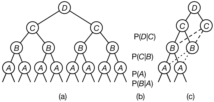
The left branch is for the variable having value false, and the right branch for the variable having value true.

Part (b) of the figure shows the stage where each factor can be evaluated. $P(D\mid C)$ can be evaluated when $D$ and $C$ are assigned values. $P(C\mid B)$ can be evaluated when $D$ , $C$ , and $B$ have been assigned values. For this variable ordering, all variables need to be split before $P(A)$ and $P(B\mid A)$ can be evaluated.

Consider the first recursive call after $D$ and $C$ have been assigned false, and $P(D\mid C)$ has been evaluated:

prob\_dfs(\{D{\,{=}\,}false,C{\,{=}\,}false\},\{P(C\mid B),P(B\mid A),P(A)\}).

Notice that the factors do not involve $D$ , and so this call will have the same value as when the context is $\{D{\,{=}\,}true,C{\,{=}\,}false\}$ .

Recursive conditioning “forgets” $D$ , and stores the computed value for

prob\_dfs(\{C{\,{=}\,}false\},\{P(C\mid B),P(B\mid A),P(A)\})

in a cache (a dictionary), and then retrieves that value for the $D{\,{=}\,}true$ case.

Similarly, after $D$ , $C$ , and $B$ have been assigned a value, the factors are $\{P(B\mid A),P(A)\}$ , which will give the same values for $C{\,{=}\,}true$ as for $C{\,{=}\,}false$ . Again, recursive conditioning saves the result of $prob\_dfs(\{B{\,{=}\,}false\},\{P(B\mid A),P(A)\})$ in a cache and retrieves that value for the other value of $C$ .

This results in the search space of Figure 9.11(c), where the dashed lines indicate a cache lookup.

Example 9.25.

Consider the query $P(B\mid d)$ for the belief network in Example 9.23. The assigned value, $D{\,{=}\,}true$ , is given as the initial context. After $B$ is assigned a value (which is needed for the denominator of Equation 9.4), the naive search algorithm has the recursive call

prob\_dfs(\{B{\,{=}\,}false,D{\,{=}\,}true\},\{P(D\mid C),P(C\mid B),P(B\mid A% ),P(A)\}).

This can be decomposed into two independent problems, one using the factors $P(D\mid C),P(C\mid B)$ , which has the same value independently of the assignment to $A$ , and the other for the factors $P(B\mid A),P(A)$ , which has the same value independently of the assignment to $C$ . These factors only have $B$ in common, which has been assigned a value in the context.

Thus, this call can be decomposed into the product:

	$\displaystyle prob\_dfs$	$\displaystyle(\{B{\,{=}\,}false,D{\,{=}\,}true\},\{P(D\mid C),P(C\mid B)\})$
		$\displaystyle\mbox{}*prob\_dfs(\{B{\,{=}\,}false,D{\,{=}\,}true\},\{P(B\mid A)% ,P(A)\}).$

1: procedure prob_RC(

{Con},{Fs}

)

2: Inputs

{Con}

: context

{Fs}

: set of factors

5: Output

\displaystyle\sum_{v_{1},\dots,v_{k}}\,\prod_{f\in{Fs}}f_{Con}

where

\{v_{1},\dots,v_{k}\}=vars({Fs})\setminus vars({Con})

7: if

({Con},{Fs})

c a c h e

with value

v

then

8: return

v

9: else if there is

X{\,{=}\,}v

{Con}

such that

X\not\in vars({Fs})

then

10: return

{prob\_RC}(\{X{\,{=}\,}v\in{Con}:X\in vars({Fs})\},{Fs}

)

11: else if

fs=\{f\in{Fs}:f\mbox{ can be evaluated in }{Con}\}

is not empty then

12: return

\left(\prod_{f\in fs}eval(f,{Con})\right)*prob\_RC({Con},{Fs}\setminus{fs})

13: else if

Fs=Fs_{1}\uplus Fs_{2}

where

vars(Fs_{1})\cap vars(Fs_{2})

are all assigned in Con then

14: return

prob\_RC({Con},Fs_{1})*prob\_RC({Con},Fs_{2})

15: else

16: select variable

v a r

vars(Fs)\setminus vars({Con})

17:

sum:=0

18: for

v a l

domain(var)

19:

sum:=sum+prob\_RC({Con}\cup\{var{\,{=}\,}val\},{Fs})

20: add

({Con},{Fs})

to cache with value

s u m

21: return

s u m

Figure 9.12: Recursive conditioning algorithm

The recursive conditioning algorithm is shown in Figure 9.12.

The function $v a r s$ returns the set of variables, as described previously for the naive algorithm.

The cache is a global dictionary that can be reused through recursive calls. It remembers what has already been computed. The keys are $({Con},{Fs})$ pairs. In order to cover the base case, the cache is initialized to have value 1 for the key $(\{\},\{\})$ .

The first condition (line 7) is to check whether the answer has already been computed and stored in the cache. If it has, the stored value is returned. Note that because of the initialization of the cache, this can replace the base case for the naive search.

The second condition (line 9) checks whether there are variables in the context that are not in any factors, and “forgets” them. This is needed so that the caching works properly, as in Example 9.24.

The third condition (line 11) checks whether some factors can be evaluated in the given context. If so, these factors are evaluated and removed from the factors of the recursive call.

The fourth condition (line 13) checks whether the problem can be split into independent parts that can be solved separately and multiplied. Here $\uplus$ is the disjoint union, where ${Fs}=Fs_{1}\uplus Fs_{2}$ means that non-empty sets $Fs_{1}$ and $Fs_{2}$ have no element in common and together contain all of the elements of ${Fs}$ . Thus, $Fs_{1}$ and $Fs_{2}$ are a partition of ${Fs}$ . If all of the variables in common are assigned in the context, the problem can be decomposed into two independent problems. The algorithm could, alternatively, split into multiple nonempty sets of factors that have no unassigned variables in any pair. They would then be the connected components, where the two factors are connected if they both contain a variable that is not assigned in the context. If there are more than two connected components, the algorithm of Figure 9.12 would find the connected components in recursive calls. Note that the subsequent recursive calls typically result in forgetting the variables that are only in the other partition, so it does not need to be done explicitly here.

If none of the other conditions hold (line 15), the algorithm branches. It selects a variable, and sums over all of the values of this variable. Which variable is selected does not affect the result, but can affect the efficiency. Finding the optimal variable to select is an NP-hard problem. Often the algorithm is given a split-order of variables in the order they should be branched on. The algorithm saves the computed result in the cache.

Examples of the application of recursive conditioning are given in Example 9.24 and Example 9.25.

Example 9.26.

Consider Example 9.13 with the query

P(Tampering\mid Smoke{\,{=}\,}true\land Report{\,{=}\,}true).

The initial call (using abbreviated names, and lower-case letters for true value) for the $Ta{\,{=}\,}false$ case is

prob\_RC(\{sm,re,\neg ta\},\{P(Ta),P(Fi),P(Al\mid Ta,Fi),P(Sm\mid Fi),P(Le\mid Al% ),P(Re\mid Le)\}).

$P(Ta)$ can be evaluated. If it then splits on $L e$ , the call is

prob\_RC(\{sm,re,\neg ta,\neg le\},\{P(Fi),P(Al\mid Ta,Fi),P(Sm\mid Fi),P(Le% \mid Al),P(Re\mid Le)\}).

At this stage $P(Re\mid Le)$ can be evaluated, and then $R e$ is not in the remaining factors, so $r e$ can be forgotten in the context. If it then splits on $A l$ , the call is

prob\_RC(\{sm,\neg ta,\neg le,\neg al\},\{P(Fi),P(Al\mid Ta,Fi),P(Sm\mid Fi),P% (Le\mid Al)\}).

Then $P(Le\mid Al)$ can be evaluated, and $\neg le$ forgotten. Splitting on $F i$ results in the call

prob\_RC(\{sm,\neg ta,\neg al,\neg fi\},\{P(Fi),P(Al\mid Ta,Fi),P(Sm\mid Fi)\}).

All of the factors can be evaluated, and so this call returns the value $P(\neg fi)*P(\neg al\mid\neg ta,\neg fi)*P(sm\mid\neg fi)$ .

The search continues; where the variables are forgotten, the cache is used to look up values rather than computing them. This can be summarized as

Variable Split on	Factors Evaluated	Forgotten
$T a$	$P(Ta)$
$L e$	$P(Re\mid Le)$	$R e$
$A l$	$P(Le\mid Al)$	$L e$
$F i$	$P(Fi)$ , $P(Al\mid Ta,Fi)$ , $P(Sm\mid Fi)$

Different variable orderings can result in quite different evaluations, for example, for the same query $P(Ta\mid sm,re)$ , for the splitting order $T a$ , $F i$ , $A l$ , $L e$ :

Variable Split on	Factors Evaluated	Forgotten
$T a$	$P(Ta)$
$F i$	$P(Fi)$ , $P(Sm\mid Fi)$	$S m$
$A l$	$P(Al\mid Ta,Fi)$	$F i$ , $T a$
$L e$	$P(Le\mid Al)$ , $P(Re\mid Le)$

If $A l$ was split before $F i$ and $L e$ , there are two independent subproblems that can be solved separately; subproblem 1 involving $F i$ and subproblem 2 involving $L e$ :

Variable Split on	Factors Evaluated	Forgotten
$T a$	$P(Ta)$
$A l$
subproblem 1:
$F i$	$P(Fi)$ , $P(Sm\mid Fi)$ , $P(Al\mid Ta,Fi)$	$S m$ , $F i$
subproblem 2:
$L e$	$P(Le\mid Al)$ , $P(Re\mid Le)$	$L e$ , $R e$

The solutions to the subproblems are multiplied.

Some of the conditions checked in Figure 9.12 only depend on the variables in the context, and not on the values of the variables. The results of these conditions can be precomputed and looked up during the search, saving a lot of time.

Some representations of factors (e.g., tables or logistic regression) require all variables to be assigned before they can be evaluated, whereas other representations (e.g., decision trees or weighted logical formula) can often be evaluated before all variables involved have been assigned values. To exploit this short-circuiting effectively, there needs to be good indexing to determine which factors can be evaluated.

9.5.2 Variable Elimination for Belief Networks

Variable elimination (VE) is the dynamic programming variant of recursive conditioning. Consider the decomposition of probability of the query $Q$ and the evidence $e$ (Equation 9.5, reproduced here):

p(Q,e)=\sum_{Z_{1}}\cdots\sum_{Z_{k}}\prod_{i=1}^{n}P(X_{i}\mid parents(X_{i})% )_{e}.

VE carries out the rightmost sum, here $\sum_{Z_{k}}$ first, eliminating $Z_{k}$ , producing an explicit representation of the resulting factor. The resulting factorization then contains one fewer variables. This can be repeated until there is an explicit representation of $P(Q,e)$ . The resulting factor is a function just of $Q$ ; given a value for $Q$ , it evaluates to a number that is the probability of the evidence conjoined with the value for $Q$ . The conditional probability can be obtained by normalization (dividing each value by the sum of the values).

To compute the posterior distribution of a query variable given observations:

1.

Construct a factor for each conditional probability distribution.
2.
Eliminate each of the non-query variables:
- •
  
  if the variable is observed, its value is set to the observed value in each of the factors in which the variable appears
- •
  
  otherwise, the variable is summed out.
  
  To sum out a variable $Z$ from a product $f_{1},\ldots,f_{k}$ of factors, first partition the factors into those not containing $Z$ , say $f_{1},\ldots,f_{i}$ , and those containing $Z$ , $f_{i+1},\ldots,f_{k}$ ; then distribute the common factors out of the sum:
  
  $\sum_{Z}\>f_{1}*\cdots*f_{k}=f_{1}*\cdots*f_{i}*\left(\sum_{Z}\>f_{i+1}*\cdots% *f_{k}\right).$
  
  Variable elimination explicitly constructs a representation (in terms of a multidimensional array, a tree, or a set of rules) of the rightmost factor. We have then simplified the problem to have one fewer variable.
3.

Multiply the remaining factors and normalize.

1: procedure VE_BN(

V s, P s, e, Q

)

2: Inputs

V s

: set of variables

P s

: set of factors representing the conditional probabilities

e

: the evidence, a variable-value assignment to some of the variables

Q

: a query variable

7: Output

8: posterior distribution on

Q

Fs\;{:}{=}\;\mbox{}Ps

\triangleright

F s

is the current set of factors

10: for each

X\in Vs-\{Q\}

using some elimination ordering do

11: if

X

is observed then

12: for each

F\in Fs

that involves

X

13: assign

X

F

to its observed value in

e

14: else

15:

Rs\;{:}{=}\;\mbox{}\{F\in Fs:F\mbox{ involves }X\}

16: let

T

be the product of the factors in

R s

17: construct an explicit representation for

N=\sum_{X}T

18:

Fs\;{:}{=}\;\mbox{}Fs\setminus Rs\cup\{N\}

19: let

T

be the product of the factors in

F s

20:

N\;{:}{=}\;\mbox{}\sum_{Q}T

21: return

T/N

Figure 9.13: Variable elimination for belief networks

Figure 9.13 gives pseudocode for the VE algorithm. The elimination ordering could be given a priori or computed on the fly. This algorithm assigns the values to the observations as part of the elimination. It is worthwhile to select observed variables first in the elimination ordering, because eliminating these simplifies the problem.

This algorithm assumes that the query variable is not observed. If it is observed to have a particular value, its posterior probability is just 1 for the observed value and 0 for the other values.

Example 9.27.

Consider Example 9.13 with the query

P(Tampering\mid Smoke{\,{=}\,}true\land Report{\,{=}\,}true).

Suppose it first eliminates the observed variables, $S m o k e$ and $R e p o r t$ . This created a factor for $P(Smoke{\,{=}\,}yes\mid Fire)$ which is just a function of $F i r e$ ; call it $f_{0}(Fire)$ . Given a value for $F i r e$ , this evaluates to a number. $P(Report{\,{=}\,}yes\mid Leaving)$ becomes a factor $f_{1}(Leaving)$ .

Suppose $F i r e$ is next in the elimination ordering. To eliminate $F i r e$ , collect all of the factors containing $F i r e$ , namely $P(Fire)$ , $P(Alarm\mid Tampering,Fire)$ , and $f_{0}(Fire)$ , and replace them with an explicit representation of the resulting factor. This factor is on $T a m p e r i n g$ and $A l a r m$ as these are the other variables in the factors being multiplied. Call it $f_{2}(Tampering,Alarm)$ :

\displaystyle f_{2}(Tampering,Alarm)

\displaystyle=\sum_{Fire}P(Fire)*(Alarm\mid Tampering,Fire)*f_{0}(Fire).

We explicitly store a number for each value for $T a m p e r i n g$ and $A l a r m$ . For example, $f_{2}(Tampering{\,{=}\,}t$ , $Alarm{\,{=}\,}f)$ has value

\sum_{v\in domain(Fire)}P(Fire{\,{=}\,}v)*P(Alarm{\,{=}\,}f\mid Tampering{\,{=% }\,}t,Fire{\,{=}\,}v)*f_{0}(Fire{\,{=}\,}v).

At this stage, $F s$ contains the factors

P(Tampering),P(Leaving\mid Alarm),f_{1}(Leaving),f_{2}(Tampering,Alarm).

Suppose $A l a r m$ is eliminated next. VE multiplies the factors containing $A l a r m$ and sums out $A l a r m$ from the product, giving a factor, call it $f_{7}$ :

f_{3}(Tampering,Leaving)=\sum_{Alarm}P(Leaving\mid Alarm)*f_{2}(Tampering,% Alarm).

$F s$ then contains the factors

\begin{array}[]{l}P(Tampering),f_{1}(Leaving),f_{3}(Tampering,Leaving).\end{array}

Eliminating $L e a v i n g$ results in the factor

f_{4}(Tampering)=\sum_{Leaving}f_{1}(Leaving)*f_{3}(Tampering,Leaving).

The posterior distribution over $T a m p e r i n g$ is given by

\frac{P(Tampering)*f_{4}(Tampering)}{\sum_{Tampering}P(Tampering)*f_{4}(% Tampering)}~{}.

Note that the denominator is the prior probability of the evidence, namely $P(Smoke{\,{=}\,}true\land Report{\,{=}\,}true)$ .

Example 9.28.

Consider the same network as in the previous example but with the query

P(Alarm\mid Fire{\,{=}\,}true).

When $F i r e$ is eliminated, the factor $P(Fire)$ becomes a factor of no variables; it is just a number, $P(Fire{\,{=}\,}true)$ .

Suppose $R e p o r t$ is eliminated next. It is in one factor, which represents $P(Report\mid Leaving)$ . Summing over all of the values of $R e p o r t$ gives a factor on $L e a v i n g$ , all of whose values are 1. This is because $P(Report{\,{=}\,}true\mid Leaving{\,{=}\,}v)+P(Report{\,{=}\,}false\mid Leaving% {\,{=}\,}v)=1$ for any value $v$ of $L e a v i n g$ .

If $L e a v i n g$ is eliminated next, a factor that is all 1 is multiplied by a factor representing $P(Leaving\mid Alarm)$ and $L e a v i n g$ is summed out. This, again, results in a factor all of whose values are 1.

Similarly, eliminating $S m o k e$ results in a factor of no variables, whose value is $1$ . Note that even if smoke had also been observed, eliminating $S m o k e$ would result in a factor of no variables, which would not affect the posterior distribution on $A l a r m$ .

Eventually, there is only the factor on $A l a r m$ that represents its posterior probability and a constant factor that will cancel in the normalization.

9.5.3 Exploiting Structure and Compilation

When the ordering of the splits in recursive conditioning is the reverse of the elimination ordering of variable elimination, the two algorithms carry out the same multiplications and additions, and the values stored in the factors of variable elimination are the same numbers as stored in the cache of recursive conditioning. The main differences are:

•

Recursive conditioning just evaluates the input factors, whereas variable elimination requires an explicit representation of intermediate factors. This means that recursive conditioning can be used where the conditional probabilities can be treated as black boxes that output a value when enough of their variables are instantiated. Thus, recursive conditioning allows for diverse representations of conditional probabilities, such as presented in Section 9.3.3. This also enables it to exploit structure when all of the variables need not be assigned. For example, in a decision tree representation of a conditional probability, it is possible to evaluate a factor before all values are assigned.
•

A straightforward implementation of variable elimination can use a more space-efficient tabular representation of the intermediate factors than a straightforward implementation of the cache in recursive conditioning.
•

When there are zeros in a product, there is no need to compute the rest of the product. Zeros arise from constraints where some combination of values to variables is impossible. This is called determinism. Determinism can be incorporated into recursive conditioning in a straightforward way.
•

Recursive conditioning can act as an any-space algorithm, which can use any amount of space by just not storing some values in the cache, but instead recomputing them, trading off space for time.

To speed up the inference, variables that are irrelevant to a conditional probability query can be pruned. In particular, any node that has no observed or queried descendants and is itself not observed or queried may be pruned. This may result in a smaller network with fewer factors and variables. For example, to compute $P(Alarm\mid Fire{\,{=}\,}true)$ , in the running example, the variables $R e p o r t$ , $L e a v i n g$ , and $S m o k e$ may be pruned.

The complexity of the algorithms depends on a measure of complexity of the network. The size of a tabular representation of a factor is exponential in the number of variables in the factor. The treewidth of a network for an elimination ordering is the maximum number of variables in a factor created by variable elimination summing out the variables in the elimination ordering. The treewidth of a belief network is the minimum treewidth over all elimination orderings. The treewidth depends only on the graph structure and is a measure of the sparseness of the graph. The complexity of recursive conditioning and variable elimination is exponential in the treewidth and linear in the number of variables. Finding the elimination ordering with minimum treewidth is NP-hard, but there are some good elimination ordering heuristics, as discussed for CSP VE.

Example 9.29.

Consider the belief network of Figure 9.4. To compute the probability of $S n e e z i n g$ , the variables $F e v e r$ and $"Achoo"~{}sound$ may be pruned, as they have no children and are not observed or queried. Summing out $S e a s o n$ involves multiplying the factors

P(Season),P(Pollen\mid Season),P(Influenza\mid Season)

and results in a factor on $I n f l u e n z a$ and $P o l l e n$ . The treewidth of this belief network is 2; there is an ordering of the variables that only constructs factors of size 1 or 2, and there is no ordering of the variables that has a smaller treewidth.

Many modern exact algorithms compile the network into a secondary structure, by essentially carrying out variable elimination or recursive conditioning symbolically, summing out all of the variables, to produce a probabilistic circuit that just contains the symbolic variables combined by sum and product. The circuit is like Figure 9.11, where the branches in (c) form the sums and the conditional probabilities in (b) are multiplied at the appropriate place, as in the factorization of Example 9.22. The circuit is an arithmetic expression with shared structure. When all variables are summed out, the circuit provides an expensive way to compute the value 1. When some variables are observed, the circuit uses the observed values instead of summing out these variables; the output is the probability of the evidence. When a query variable is then set to a value, the circuit outputs the probability of the evidence and the query variable, from which a conditional probability can be computed. It is possible to compute the posterior probability of all variables with two passes through the circuit, but that is beyond the scope of this book.

Compilation is appropriate when the same belief network is used for many multiple queries, or where observations are added incrementally. Unfortunately, extensive preprocessing, allowing arbitrary sequences of observations and deriving the posterior on each variable, precludes pruning the network. So for each application you need to choose whether you will save more by pruning irrelevant variables for each query or by preprocessing before there are any observations or queries.

Artificial Intelligence 3E

9.5 Exact Probabilistic Inference

Naive Search-Based Algorithm

Exploiting Independence in Inference

Example 9.22.

Example 9.23.

9.5.1 Recursive Conditioning

Example 9.24.

Example 9.25.

Example 9.26.

9.5.2 Variable Elimination for Belief Networks

Example 9.27.

Example 9.28.

9.5.3 Exploiting Structure and Compilation

Example 9.29.

Artificial
Intelligence 3E