7 Supervised Machine Learning 7.3 Basic Models for Supervised Learning 7.5 Composite Models

7.4 Overfitting

Overfitting occurs when the learner makes predictions based on regularities that appear in the training examples but do not appear in the test examples or in the world from which the data is taken. It typically happens when the model tries to find signal in randomness – spurious correlations in the training data that are not reflected in the problem domain as a whole – or when the learner becomes overconfident in its model. This section outlines methods to detect and avoid overfitting.

The following example shows a practical example of overfitting.

Example 7.15.

Consider a website where people submit ratings for restaurants from 1 to 5 stars. Suppose the website designers would like to display the best restaurants, which are those restaurants that future patrons would like the most. It is tempting to return the restaurants with the highest mean rating, but that does not work.

It is extremely unlikely that a restaurant that has many ratings, no matter how outstanding it is, will have a mean of 5 stars, because that would require all of the ratings to be 5 stars. However, given that 5-star ratings are not that uncommon, it would be quite likely that a restaurant with just one rating will have 5 stars. If the designers used the mean rating, the top-rated restaurants will be ones with very few ratings, and these are unlikely to be the best restaurants. Similarly, restaurants with few ratings but all low are unlikely to be as bad as the ratings indicate.

The phenomenon that extreme predictions will not perform as well on test cases is analogous to regression to the mean. Regression to the mean was discovered by Galton [1886], who called it regression to mediocrity, after discovering that the offspring of plants with larger than average seeds are more like average seeds than their parents are. In both the restaurant and the seed cases, this occurs because ratings, or the size, will be a mix of quality and luck (e.g., who gave the rating or what genes the seeds had). Restaurants that have a very high rating will have to be high in quality and be lucky (and be very lucky if the quality is not very high). More data averages out the luck; it is very unlikely that someone’s luck does not run out. Similarly, the seed offspring do not inherit the part of the size of the seed that was due to random fluctuations.

Overfitting can also be caused by model complexity: a more complex model, with more parameters, can almost always fit data better than a simple model.

Refer to caption — Figure 7.15: Fitting polynomials to the data of Figure 7.2

Example 7.16.

A polynomial of degree $k$ is of the form

y=w_{0}+w_{1}*x+w_{2}*x^{2}+\dots+w_{k}*x^{k}.

Linear regression can be used unchanged to learn the weights of the polynomial that minimize the squared error, simply by using $1,x,x^{2},\dots,x^{k}$ as the input features to predict $y$ .

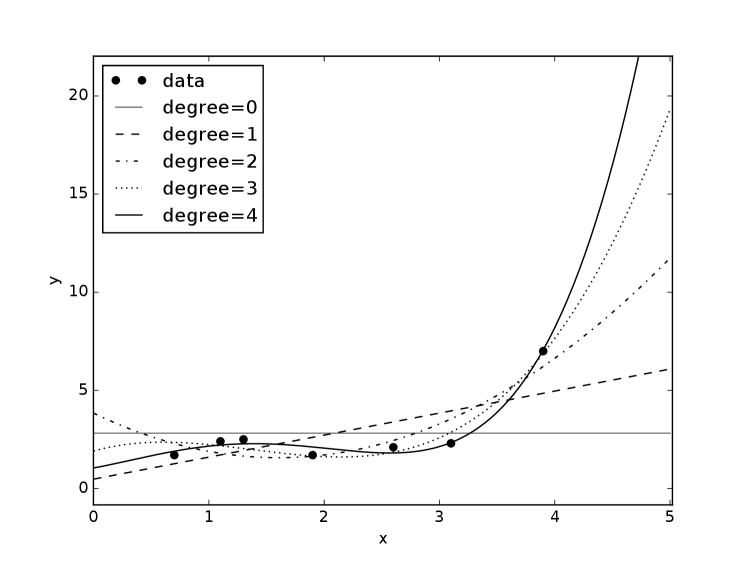
Figure 7.15 shows polynomials up to degree 4 for the data of Figure 7.2. Higher-order polynomials can fit the data better than lower-order polynomials, but that does not make them better on the test set.

Notice how the higher-order polynomials get more extreme in extrapolation. All of the polynomials, except the degree 0 polynomials, go to plus or minus infinity as $x$ gets bigger or smaller, which is almost never what you want. Moreover, if the maximum value of $k$ for which $w_{k}\neq 0$ is even, then as $x$ approaches plus or minus infinity, the predictions will have the same sign, going to either plus infinity or minus infinity. The degree-4 polynomial in the figure approaches $\infty$ as $x$ approaches $-\infty$ , which does not seem reasonable given the data. If the maximum value of $k$ for which $w_{k}\neq 0$ is odd, then as $x$ approaches plus or minus infinity, the predictions will have opposite signs.

Example 7.15 shows how more data can allow for better predictions. Example 7.16 shows how complex models can lead to overfitting the data. Given a fixed dataset, the problem arises as to how to make predictions that make good predictions on test sets.

The test set error is caused by bias, variance, and/or noise:

•

Bias, the error due to the algorithm finding an imperfect model. The bias is low when the model learned is close to the ground truth, the process in the world that generated the data. The bias can be divided into representation bias caused by the representation not containing a hypothesis close to the ground truth, and a search bias caused by the algorithm not searching enough of the space of hypotheses to find the best hypothesis. For example, with discrete features, a decision tree can represent any function, and so has a low representation bias. With a large number of features, there are too many decision trees to search systematically, and decision tree learning can have a large search bias. Linear regression, if solved directly using the analytic solution, has a large representation bias and zero search bias. There would also be a search bias if the gradient descent algorithm was used.
•

Variance, the error due to a lack of data. A more complicated model, with more parameters to tune, will require more data. Thus, with a fixed amount of data, there is a bias–variance trade-off; you can have a complicated model which could be accurate, but you do not have enough data to estimate it appropriately (with low bias and high variance), or a simpler model that cannot be accurate, but you can estimate the parameters reasonably well given the data (with high bias and low variance).
•

Noise, the inherent error due to the data depending on features not modeled or because the process generating the data is inherently stochastic.

Overfitting results in overconfidence, where the learner is more confident in its prediction than the data warrants. For example, in the predictions in Figure 7.14, trained on eight examples, the probabilities are much more extreme than could be justified by eight examples. The first prediction, that there is approximately 2% chance of $t$ being true when $x$ , $y$ , and $z$ are false, does not seem to be reasonable given only one example of this case. As the search proceeds, it becomes even more confident. This overconfidence is reflected in test error, as in the following example.

Example 7.17.

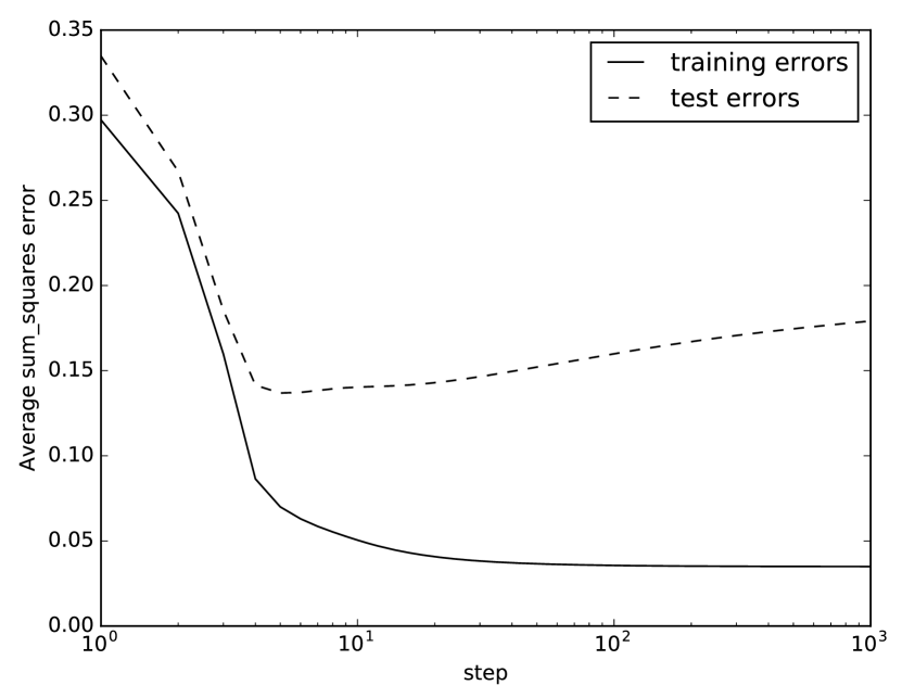
Figure 7.16 shows a typical plot of how the training and test errors change with the number of iterations of gradient descent. The error on the training set decreases as the number of iterations increases. For the test set, the error reaches a minimum and then increases as the number of iterations increases. As it overfits to the training examples, errors in the test set become bigger because it becomes more confident in its imperfect model.

The following sections discuss three ways to avoid overfitting. The first, pseudocounts, explicitly allows for regression to the mean, and can be used for cases where the representations are simple. The second, regularization, provides an explicit trade-off between model complexity and fitting the data. The third, cross validation, is to use some of the training data to detect overfitting.

7.4.1 Pseudocounts

For many of the prediction measures, the optimal prediction on the training data is the mean. In the case of Boolean data (assuming true is represented as 1, and false as 0), the mean can be interpreted as a probability. However, the empirical mean, the mean of the training set, is typically not a good estimate of the probability of new cases, as was shown in Example 7.15.

A simple way both to solve the zero-probability problem and to take prior knowledge into account is to use pseudo-examples, which are added to the given examples. The number of pseudo-examples used is a nonnegative pseudocount or prior count, which is not necessarily an integer.

Suppose the examples are values $v_{1},\dots,v_{n}$ and you want to make a prediction for the next $v$ , written as $\widehat{v}$ . When $n=0$ , assume you use prediction $a_{0}$ (which you cannot get from data as there are no data for this case). For the other cases, use

\widehat{v}=\frac{c*a_{0}+\sum_{i}v_{i}}{c+n}

where $c$ is a nonnegative real-value constant, which is the number of assumed fictional data points. This is assuming there are $c$ pseudo-examples, each with a value of $a_{0}$ . The count $c$ does not have to be an integer, but can be any nonnegative real value. If $c=0$ , the prediction is the mean value, but that prediction cannot be used when there is no data (when $n=0$ ). The value of $c$ controls the relative importance of the initial hypothesis (the prior) and the data.

Example 7.18.

Consider how to better estimate the ratings of restaurants in Example 7.15. The aim is to predict the mean rating over the test data, not the mean rating of the seen ratings.

You can use the existing data about other restaurants to make estimates about the new cases, assuming that the new cases are like the old. Before seeing anything, it may be reasonable to use the mean rating of the restaurants as the value for $a_{0}$ . This would be like assuming that a new restaurant is like an average restaurant (which may or may not be a good assumption). Suppose you are most interested in being accurate for top-rated restaurants. To estimate $c$ , consider a restaurant with a single 5-star rating. You could expect this rating to be like other 5-star ratings. Let $a^{\prime}$ be the mean rating of the restaurants with 5-star ratings (where the mean is weighted by the number of 5-star ratings each restaurant has). This is an estimate of the restaurant quality for a random 5-star rating by a user, and so may be reasonable for the restaurant with a single 5-star rating. In the equation above, with $n=1$ and $\sum_{i}v_{i}=5$ , this gives $a^{\prime}=(c*a_{0}+5)/(c+1)$ . Solving for $c$ gives $c=(5-a^{\prime})/(a^{\prime}-a_{0})$ .

Suppose the mean rating for all restaurants ( $a_{0}$ ) is $3$ , and the mean rating for the restaurants with a 5-star rating $a^{\prime}$ is 4.5. Then $c=1/3$ . If the mean for restaurants with 5-star ratings was instead 3.5, then $c$ would be 3. See Exercise 7.13.

Section 17.2.1 shows how to do better than this by taking into account the other ratings of the person giving the rating.

Consider the following thought experiment (or, better yet, implement it):

•

Select a number $p$ at random uniformly from the range $[0,1]$ . Suppose this is the ground truth for the probability that $Y=1$ for a variable $Y$ with domain $\{0,1\}$ .
•

Generate $n$ training examples with $P(Y{\,{=}\,}1)=p$ . To do this, for each example, generate by a random number uniformly in range $[0,1)$ , and record $Y{\,{=}\,}1$ if the random number is less than $p$ , and $Y{\,{=}\,}0$ otherwise. Let $n_{1}$ be the number of examples with $Y{\,{=}\,}1$ and so there are $n_{0}=n-n_{1}$ samples with $Y{\,{=}\,}0$ .
•

Generate some (e.g., 10) test cases with the same $p$ .

The learning problem for this scenario is: from $n_{0}$ and $n_{1}$ create the estimator $\widehat{p}$ with the smallest error on the test cases. If you try this for a number of values of $n$ , such as $1,2,3,4,5,10,20,100,1000$ and repeat this 1000 times, you will get a good idea of what is going on.

With squared error or log loss, you will find that the empirical mean $\widehat{p}=n_{1}/(n_{0}+n_{1})$ , which has the smallest error on the training set, works poorly on the test set, with the log loss typically being infinity. The log loss is infinity when one of 0 or 1 does not appear in the training set (so the corresponding $n_{i}$ is zero) but appears in the test set.

Laplace smoothing, defined by $\widehat{p}=(n_{1}+1)/(n_{0}+n_{1}+2)$ , has the smallest log loss and squared error of all estimators on the test set. This is equivalent to two pseudo-examples: one of 0 and one of 1. A theoretical justification for Laplace smoothing is presented in Section 10.2. If $p$ were selected from some distribution other than the uniform distribution, Laplace smoothing may not result in the best predictor.

7.4.2 Regularization

Ockham’s razor specifies that you should prefer simpler hypotheses over more complex ones. William of Ockham was an English philosopher who was born in about 1285 and died, apparently of the plague, in 1349. (Note that “Occam” is the French spelling of the English town “Ockham” and is often used.) He argued for economy of explanation: “What can be done with fewer [assumptions] is done in vain with more.”

An alternative to optimizing fit-to-data is to optimize fit-to-data plus a term that rewards model simplicity and penalizes complexity. The penalty term is a regularizer.

The typical form for a regularizer is to find a predictor $\widehat{Y}$ to minimize

\left(\sum_{e}loss(\widehat{Y}({e}),{Y}({e}))\right)+\lambda*regularizer(% \widehat{Y})

(7.5)

where $loss(\widehat{Y}({e}),{Y}({e}))$ is the loss of example $e$ for predictor $\widehat{Y}$ , which specifies how well $\widehat{Y}$ fits example $e$ , and $regularizer(\widehat{Y})$ is a penalty term that penalizes complexity. The regularization parameter, $\lambda$ , trades off fit-to-data and model simplicity. As the number of examples increases, the leftmost sum tends to dominate and the regularizer has little effect. The regularizer has most effect when there are few examples. The regularization parameter is needed because the error and complexity terms are typically in different units.

A hyperparameter is a parameter used to define what is being optimized, or how it is optimized. It can be chosen by prior knowledge, past experience with similar problems, or hyperparameter tuning to choose the best values using cross validation.

The regularization parameter, $\lambda$ above, is a hyperparameter. In learning a decision tree one complexity measure is the number of leaves in a decision tree (which is one more than the number of splits for a binary decision tree). When building a decision tree, you could optimize the sum of a loss plus a function of the size of the decision tree, minimizing

\left(\sum_{e\in E}loss(\widehat{Y}({e}),{Y}({e}))\right)+\gamma*|tree|

where $|tree|$ is the number of leaves in a tree representation of $\widehat{Y}$ . This uses $\gamma$ instead of $\lambda$ , following the convention in gradient-boosted trees (see below). A single split on a leaf increases the number of leaves by 1. When splitting, a single split is worthwhile if it reduces the sum of losses by $\gamma$ . This regularization is implemented in the decision tree learner (Figure 7.9).

For models where there are real-valued parameters, an L2 regularizer penalizes the sum of squares of the parameters. To optimize the squared error for linear regression with an $L2$ regularizer, minimize

\displaystyle\left(\sum_{e\in E}\left({Y}({e})-\sum_{i=0}^{m}w_{i}*{X_{i}}({e}% )\right)^{2}\right)+\lambda\left(\sum_{i=0}^{m}w_{i}^{2}\right)

which is known as ridge regression. Note that this is equivalent to $\lambda$ pseudo-examples with a value of $0$ for the target, and a value of 1 for each input feature.

It is possible to use multiple regularizers, for example including both $\gamma$ for tree size and $\lambda$ for $L2$ regularization.

To optimize the log loss error for logistic regression with an $L2$ regularizer, minimize

\displaystyle-\left(\sum_{e\in E}\left({Y}({e})\log\widehat{Y}({e})+(1-{Y}({e}% ))\log(1-\widehat{Y}({e}))\right)\right)+\lambda\left(\sum_{i=0}^{m}w_{i}^{2}\right)

where $\widehat{Y}({e})=sigmoid\left(\sum_{i=0}^{m}w_{i}*{X_{i}}({e})\right)$ .

An $L2$ regularization is implemented for stochastic gradient descent by adding

\displaystyle w_{i}

\displaystyle\;{:}{=}\;\mbox{}w_{i}-\eta*\lambda*b/|E|*w_{i}

after line 24 of Figure 7.12 (in the scope of “for each”). The $b/|E|$ is because the regularization is $\lambda$ for the whole dataset, but the update occurs for each batch of size $b$ . Note that $\eta*\lambda*b/|E|$ changes rarely, if ever, and so can be stored until one of its constituents change.

An L1 regularizer adds a penalty for the sum of the absolute values of the parameters.

To optimize the squared error for linear regression with an $L1$ regularizer, minimize

\displaystyle\left(\sum_{e\in E}\left({Y}({e})-\sum_{i=0}^{m}w_{i}*{X_{i}}({e}% )\right)^{2}\right)+\lambda\left(\sum_{i=0}^{m}|w_{i}|\right)

which is called lasso (least absolute shrinkage and selection operator).

Adding an $L1$ regularizer to the log loss entails minimizing

\displaystyle-\left(\sum_{e\in E}\left({Y}({e})\log\widehat{Y}({e})+(1-{Y}({e}% ))\log(1-\widehat{Y}({e}))\right)\right)+\lambda\left(\sum_{i=0}^{m}\left|w_{i% }\right|\right).

The partial derivative of the sum of absolute values with respect to $w_{i}$ is the sign of $w_{i}$ , either $1$ or $-1$ (defined as $sign(w_{i})=w_{i}/|w_{i}|$ ), at every point except at 0. You do not need to make a step at 0, because the value is already a minimum. To implement an $L1$ regularizer, each parameter is moved towards zero by a constant, except if that constant would change the sign of the parameter, in which case the parameter becomes zero. An $L1$ regularizer can be incorporated into the gradient descent algorithm of Figure 7.12 by adding after line 24 (in the scope of “for each”):

\displaystyle w_{i}\;{:}{=}\;\mbox{}sign(w_{i})*max(0,\>|w_{i}|-\eta*\lambda*b% /|E|).

This is called iterative soft-thresholding and is a special case of the proximal-gradient method.

$L1$ regularization with many features tends to make many weights zero, which means the corresponding feature is ignored. This is a way to implement feature selection. An $L2$ regularizer tends to make all of the parameters smaller, but not zero.

7.4.3 Cross Validation

The problem with the previous methods is that they require a notion of simplicity to be known before the agent has seen any data. It would seem that an agent should be able to determine, from the training data, how complicated a model needs to be. Such a method could be used when the learning agent has no prior information about the world.

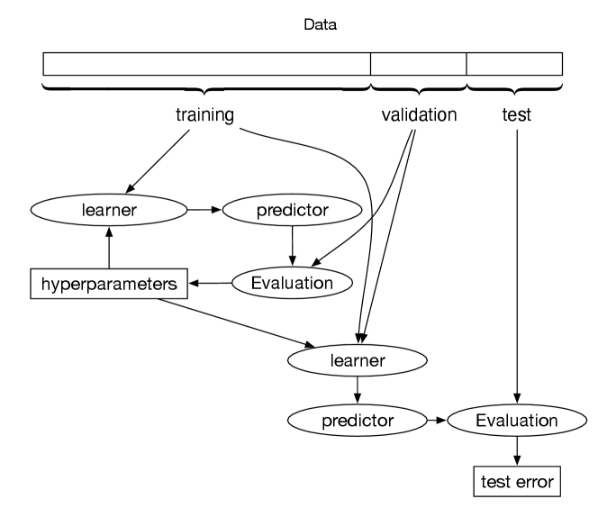
Figure 7.17 shows a general pattern for learning and evaluating learning algorithms. Recall that you need to remove some of the examples as the test set and only ever use these for the final evaluation. The aim is to predict examples that the agent has not seen, and the test set acts as a surrogate for these unseen examples, and so cannot be used in any part of training.

The idea of cross validation is to use part of the non-test data as a surrogate for test data. In the simplest case, split the non-test data into two: a set of examples to train with, and a validation set, also called the dev (development) set or holdout. The agent uses the remaining examples as the training set to build models. The validation set can act as a surrogate for the test set in evaluating the predictions from the training set.

The evaluation of the validation set is used to choose hyperparameters of the learner. The hyperparameters are any choices that need to be made for the learner, including the choice of the learning algorithm, the values of regularization parameters, and other choices that affect the model learned.

Once the hyperparameters have been set, the whole non-test dataset can be used to build a predictor, which is evaluated on the test set.

To see how the validation error could be used, consider a graph such as the one in Figure 7.16, but where the test errors instead come from the validation set. The error on the training set gets smaller as the size of the tree grows. However, on the validation set (and the test set), the error typically improves for a while and then starts to get worse. The idea of cross validation is to choose a parameter setting or a representation in which the error of the validation set is a minimum. The hyperparameter here is how many steps to train for before returning a predictor. This is known as early stopping. The hypothesis is that the parameter setting where the validation set is a minimum is also where the error on the test set is a minimum.

Typically, you want to train on as many examples as possible, because then you get better models. However, a larger training set results in a smaller validation set, and a small validation set may or may not fit well just by luck.

To overcome this problem for small datasets, $k$ -fold cross validation allows examples to be used for both training and validation, but still use all of the data for the final predictor. It has the following steps:

•

Partition the non-test examples randomly into $k$ sets, of approximately equal size, called folds.
•

To evaluate a parameter setting, train $k$ times for that parameter setting, each time using one of the folds as the validation set and the remaining folds for training. Thus each fold is used as a validation set exactly once. The accuracy is evaluated using the validation set. For example, if $k=10$ , then 90% of the training examples are used for training and 10% of the examples for validation. It does this 10 times, so each example is used once in a validation set.
•

Optimize parameter settings based on the error on each example when it is used in the validation set.
•

Return the model with the selected parameter settings, trained on all of the data.

Example 7.19.

One of the possible hyperparameters for the decision tree learner is the minimum number of examples that needs to be in a child, so the stopping criterion for the decision tree learner of Figure 7.9 will be true if the number of examples in a child is less than $min\_child\_size$ . If this threshold is too small, the decision tree learner will tend to overfit, and if it is too large, it will tend not to generalize.

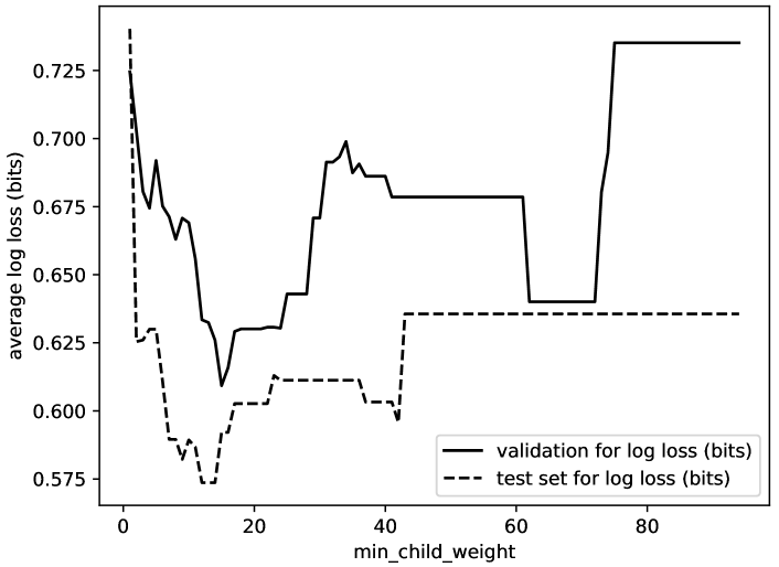
Figure 7.18 shows the validation error for 5-fold cross validation as a function of the hyperparameter $min\_child\_size$ . For each point on the $x$ -axis, the decision tree was run five times, and the mean log loss was computed for the validation set. The error is at a minimum at 39, and so this is selected as the best value for this parameter. This plot also shows the error on the test set for trees with various settings for the minimum number of examples, and 39 is a reasonable parameter setting based on the test set. A learner does not get to see the error on the test set when selecting a predictor.

At one extreme, when $k$ is the number of training examples, $k$ -fold cross validation becomes leave-one-out cross validation. With $m$ examples in the training set, it learns $m$ times; for each example $e$ , it uses the other examples as training set, and evaluates on $e$ . This is not practical if each training is done independently, because it increases the complexity by the number of training examples. However, if the model from one run can be adjusted quickly when one example is removed and another added, this can be very effective.

One special case is when the data is temporal and the aim is to extrapolate; to predict the future from the past. To work as a surrogate for predicting the future, the test set should be the latest examples. The validation set can then be the examples immediately before these. The analogy to leave-one-out cross validation is to learn each example using only examples before it.

The final predictor to be evaluated on the test can use all of the non-test examples in its predictions. This might mean adjusting some of the hyperparameters to account for the different size of the final training set.

Artificial Intelligence 3E