Artificial
Intelligence 3E
foundations of computational agents
8.4 Convolutional Neural Networks
Imagine using a neural network for recognizing objects in large images using a dense network, as in Example 8.3. There are two aspects that might seem strange. First, it does not take into account any spatial locality, if the pixels were shuffled consistently in all of the images, the neural network would act the same. Humans would not be able to recognize objects any more, because humans take the spatial proximity into account. Second, it would have to learn to recognize cats, for example, separately when they appear in the bottom-left of an image and when they appear in the bottom-right and in the top-middle of an image. Convolutional neural networks tackle these problems by using filters that act on small patches of an image, and by sharing the parameters so they learn useful features no matter where in an image they occur.
In a convolutional neural network (CNN), a kernel (sometimes called a convolution mask, or filter) is a learned linear operator that is applied to local patches. The following first covers one-dimensional kernels, used for sequences such as sound or text, then two-dimensional kernels, as used in images. Higher-dimensional kernels are also used, for example in video.
In one dimension, suppose the input is a sequence (list) and there is structure so that is close to in some sense. For example, could be the th value of a speech signal in time, and is the next one in time. In a spectrum, could be the value of one frequency, and the value for the next frequency measured.
A one-dimensional kernel is a vector , where is the kernel size, which when applied to the sequence produces a sequence where
Example 8.7.
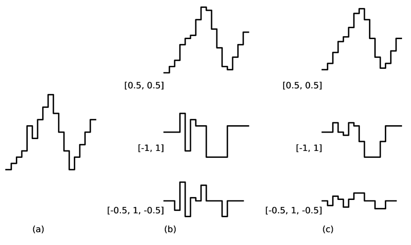
Consider the kernel . Applying this to the signal gives the sequence
shown in Figure 8.8(b), top. Each value is the mean of two adjoining values in the original signal. This kernel smooths a sequence.
Applying the kernel to the original sequence results in the sequence
which is the slope; it is positive when the value is increasing and negative when the value is decreasing. See Figure 8.8(b), middle.
The kernel finds peaks and troughs. It is positive when the value is locally higher than its neighbors, and negative when the value is lower than its neighbors. The magnitude reflects how much it is greater or less. See Figure 8.8(b), bottom.
Figure 8.8(c) shows the same kernels applied to the smoothed signal (Figure 8.8(b), top).
A two-dimensional kernel is a array , where is the kernel size, which when applied to the two-dimensional array produces a two-dimensional array where
The kernel size, , is usually much smaller than the size of either dimension of . Two-dimensional kernels are used for images, where they are applied to patches of adjacent pixels.
Example 8.8.
Consider the following kernels that could be applied to a black-and-white image where the value of is the brightness of the pixel at position :
| 0 | 1 |
| 0 | |
| (a) | |
| 1 | 0 |
| 0 | |
| (b) | |
| 0 | 1 | |
| 0 | 2 | |
| 0 | 1 | |
| (c) | ||
| 2 | 1 | |
| 0 | 0 | 0 |
| (d) | ||
Kernels (a) and (b) were invented by Roberts [1965]. The result of (a) is positive when the top-right pixel in a block is greater than the pixel one down and to the left. This can be used to detect the direction of a change in shading. Kernels (a) and (b) together can recognize various directions of the change in shading; when (a) and (b) are both positive, the brightness increases going up. When (a) is positive and (b) is negative, the brightness increases going right. When (a) is positive and (b) close to zero, the brightness increases going up-right.
Kernels (c) and (d) are the Sobel-Feldman operators for edge detection, where (c) finds edges in the -direction and (d) finds edges in the -direction; together they can find edges in other directions.
Before machine learning dominated image interpretation, kernels were hand designed to have particular characteristics. Now kernels are mostly learned.
Convolutional neural networks learn the weights for the kernels from data. Two main aspects distinguish convolutional neural networks from ordinary neural networks.
-
•
Locality: the values are a function of neighboring positions, rather than being based on all units as they are in a fully-connected layer. For example, a kernel for vision uses two pixels in each direction of a point to give a value for the point for the next layer. Multiple applications of kernels can increase the size of influence. For example, in image interpretation, when two consecutive convolutional layers use kernels, the values of the second one depend on four pixels in each direction in the original image.
-
•
Parameter sharing or weight tying means that, for a single kernel, the same parameters are used at all locations in the image.
Figure 8.9 shows the algorithm for a two-dimensional convolutional layer, where only one kernel is applied to the input array. The kernel is a square. The input is an rectangle. The output is smaller than the input, removing values from each dimension. In backpropagation, the input error () and are updated once for each time the corresponding input or weight is used to compute an output. Unlike in the dense linear function (Figure 8.3), parameter sharing means that during backpropagation each is updated multiple times for a single example.
Real convolutional neural networks are more sophisticated than this, including the following features:
-
•
The kernel does not need to be square, but can be any rectangular size. This affects the size of and .
-
•
Because the algorithm above requires each array index to be in range, it removes elements from the edges. This is problematic for deep networks, as the model eventually shrinks to zero as the number of layers increases. It is common to add zero padding: expand the input (or the output) by zeros symmetrically – with the same number of zeros on each side – so that the output is the same size as the input. The use of padding means it is reasonable for the kernel indexes to start from 0, whereas it was traditional to have them be symmetric about 0, such as in the range .
-
•
Multiple kernels are applied concurrently. This means that the output consists of multiple two-dimensional arrays, one for each kernel used. These multiple arrays are called channels. To stack these into layers, the input also needs to be able to handle multiple channels. A color image typically has three channels corresponding to the colors red, green, and blue. (Cameras for scientific purposes can contain many more channels.)
To represent multiple channels for the input and the output, the weight array, , becomes four-dimensional; one for , one for , one for the input channel, and one for the output channel. The pseudocode needs to be expanded, as follows. If the input is for input channel and the output is for output channel , there is a weight for each . In the method , there is an extra loop over , and the output assignment becomes
needs also to loop over the input channels and the output channels, updating each parameter.
Instead of all input channels being connected to all output channels, sometimes they are grouped so that only the input and output channels in the same group are connected.
-
•
The above algorithm does not include a bias term – the weight multiplied by 1. Whether to use a bias is a parameter in most implementations, with a default of using a bias.
-
•
This produces an output of the same size as the input, perhaps with a fixed number of pixels removed at the sides. It is also possible to down-sample, selecting every second (which would halve the size of each dimension) or every third value (which would divide the size of each dimension by three), for example. While this could be done with an extra layer to down-sample, it is more efficient to not compute the values to be thrown away, thus down-sampling is usually incorporated into the convolutional layer.
A stride for a dimension is a positive integer such that each th value is used in the output. For two dimensions, a stride of 2 for each dimension will halve the size of each dimension, and so the output will be a quarter the size of the input. For example, a image with a stride of 2 for each dimension will output a array, which in later layers can use another stride of 2 in each dimension to give a array. A stride of 1 selects all output values, and so is like not having a stride. There can be a separate stride for each dimension.
-
•
In a pooling layer, instead of a learnable linear kernel, a fixed function of the outputs of the units is applied in a kernel. A common pooling layer is max-pooling, which is like a convolution, but where the maximum is used instead of a linear function. Pooling is typically combined with a stride greater than 1 to down-sample as well. It is typical to use a convolution layer, followed by a nonlinear function, such as ReLU, followed by a pooling layer, the output of which is then input to a convolution layer and so on.
-
•
When used for classification of the whole image (e.g., detecting whether there is a cat or a baby in the image), a convolutional neural network typically ends with fully-connected layers. Note that to use standard fully-connected layers, the array needs to be flattened into a vector; this is done by concatenating the rows or the columns. A fully convolutional neural network has a number of convolution layers, but no fully-connected layer. This is used to classify each point in an image (e.g., whether each pixel is part of a cat or part of the background).
-
•
A shortcut connection or a skip connection in a deep network is a connection that skips some layers. In particular, some of the input channels of a layer come from the previous layer and some from lower-level layers. In a residual network, the values from one layer are added to the values from a lower layer. In this case, the intermediate layers – those between the two layers being added – become trained to predict the error, in a similar way to boosting. The first residual network [He et al., 2015] won many competitions for classification from images. One of their models had a depth of 152 layers with over a million parameters, and was trained on an ImageNet dataset with 1000 classes and 1.28 million training examples.
Artificial Intelligence: Foundations of Computational Agents, Poole
& Mackworth
Copyright © 2023, David L. Poole and Alan K. Mackworth. 
This work is licensed under a Creative Commons Attribution-NonCommercial-NoDerivatives 4.0 International License.