Artificial
Intelligence 3E
foundations of computational agents
12.5 Decision Processes
Recall that the planning horizon is how far ahead an agent considers when planning. The decision networks of Section 12.3.1 were for finite-stage, partially observable domains. This section considers indefinite-horizon and infinite-horizon problems.
Often an agent must reason about an ongoing process or it does not know how many actions it will be required to do. These are called infinite-horizon problems when the process may go on forever or indefinite-horizon problems when the agent will eventually stop, but it does not know when it will stop.
For ongoing processes, it may not make sense to consider only the utility at the end, because the agent may never get to the end. Instead, an agent can receive a sequence of rewards. Rewards provide a way to factor utility through time, by having a reward for each time, and accumulating the rewards to determine utility. Rewards can incorporate action costs in addition to any prizes or penalties that may be awarded. Negative rewards are called punishments. Indefinite-horizon problems can be modeled using a stopping state. A stopping state or absorbing state is a state in which all actions have no effect; that is, when the agent is in that state, all actions immediately return to that state with a zero reward. Goal achievement can be modeled by having a reward for entering such a stopping state.
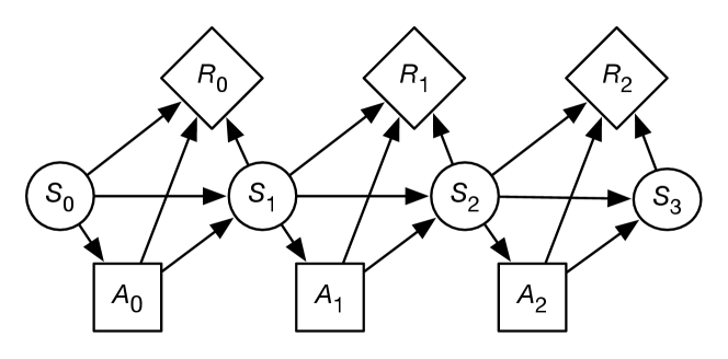
A Markov decision process can be seen as a Markov chain augmented with actions and rewards or as a decision network extended in time. At each stage, the agent decides which action to perform; the reward and the resulting state depend on both the previous state and the action performed.
Unless noted, assume a stationary model, where the state transitions and the rewards do not depend on the time.
A Markov decision process, or MDP, consists of
-
•
, a set of states of the world
-
•
, a set of actions
-
•
, which specifies the dynamics. This is written as , the probability of the agent transitioning into state given that the agent is in state and does action . Thus
-
•
, where , the reward function, gives the expected immediate reward from doing action and transitioning to state from state . Sometimes it is convenient to use , the expected value of doing in state , which is .
A finite part of a Markov decision process can be depicted using a decision network as in Figure 12.15.
Example 12.29.
Suppose Sam wanted to make an informed decision about whether to party or relax over the weekend. Sam prefers to party, but is worried about getting sick. Such a problem can be modeled as an MDP with two states, and , and two actions, and . Thus
Based on experience, Sam estimates that the dynamics is given by
| Probability of | ||
|---|---|---|
| 0.95 | ||
| 0.7 | ||
| 0.5 | ||
| 0.1 |
So, if Sam is healthy and parties, there is a 30% chance of becoming sick. If Sam is healthy and relaxes, Sam will more likely remain healthy. If Sam is sick and relaxes, there is a 50% chance of getting better. If Sam is sick and parties, there is only a 10% chance of becoming healthy.
Sam estimates the rewards to be the following, irrespective of the resulting state:
| Reward | ||
|---|---|---|
| 7 | ||
| 10 | ||
| 0 | ||
| 2 |
Thus, Sam always enjoys partying more than relaxing. However, Sam feels much better overall when healthy, and partying results in being sick more than relaxing does.
The problem is to determine what Sam should do each weekend.
Example 12.30.
A grid world is an idealization of a robot in an environment. At each time, the robot is at some location and can move to neighboring locations, collecting rewards and punishments. Suppose that the actions are stochastic, so that there is a probability distribution over the resulting states given the action and the state.
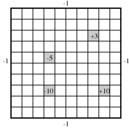
Figure 12.16 shows a grid world, where the robot can choose one of four actions: up, down, left, or right. If the agent carries out one of these actions, it has a chance of going one step in the desired direction and a chance of going one step in any of the other three directions. If it bumps into the outside wall (i.e., the location computed is outside the grid), there is a penalty of 1 (i.e., a reward of ) and the agent does not actually move. There are four rewarding states (apart from the walls), one worth (at position ; 9 across and 8 down), one worth (at position ), one worth (at position ), and one worth (at position ). In each of these states, the agent gets the reward after it carries out an action in that state, not when it enters the state. When the agent reaches one of the states with positive reward (either or ), no matter what action it performs, at the next step it is flung, at random, to one of the four corners of the grid world.
Note that the reward in this example depends on both the initial state and the final state. The agent bumped into the wall, and so received a reward of , if and only if the agent remains in the same state. Knowing just the initial state and the action, or just the final state and the action, does not provide enough information to infer the reward.
As with decision networks, the designer also has to consider what information is available to the agent when it decides what to do. There are two variations:
-
•
In a fully observable Markov decision process (MDP), the agent gets to observe the current state when deciding what to do.
-
•
A partially observable Markov decision process (POMDP) is a combination of an MDP and a hidden Markov model (HMM). At each time, the agent gets to make some (ambiguous and possibly noisy) observations that depend on the state. The agent only has access to the history of rewards, observations, and previous actions when making a decision. It cannot directly observe the current state.
Rewards
To decide what to do, the agent compares different sequences of rewards. The most common way to do this is to convert a sequence of rewards into a number called the return, the cumulative reward, or the value. This is a number that specifies the utility to an agent of the current and future rewards. To compute the return, the agent combines the current reward with other rewards in the future. Suppose the agent receives the sequence of rewards
Three common reward criteria are used to combine rewards into a value :
- Total reward
-
. In this case, the value is the sum of all of the rewards. This works when you can guarantee that the sum is finite; but if the sum is infinite, it does not give any opportunity to compare which sequence of rewards is preferable. For example, a sequence of 1 rewards has the same total as a sequence of 100 rewards (both are infinite). One case where the total reward is finite is when there are stopping states and the agent always has a non-zero probability of eventually entering a stopping state.
- Average reward
-
. In this case, the agent’s value is the average of its rewards, averaged over for each time period. As long as the rewards are finite, this value will also be finite. However, whenever the total reward is finite, the average reward is zero, and so the average reward will fail to allow the agent to choose among different actions that each have a zero average reward. Under this criterion, the only thing that matters is where the agent ends up. Any finite sequence of bad actions does not affect the limit. For example, receiving 1,000,000 followed by rewards of 1 has the same average reward as receiving 0 followed by rewards of 1 (they both have an average reward of 1).
- Discounted reward
-
, where , the discount factor, is a number in the range . Under this criterion, future rewards are worth less than the current reward. If was 1, this would be the same as the total reward. When , the agent ignores all future rewards. Having guarantees that, whenever the rewards are finite, the total value will also be finite.
The discounted reward can be rewritten as
Suppose is the reward accumulated from time :
To understand the properties of , suppose , then . Solving for gives . Thus, with the discounted reward, the value of all of the future is at most times as much as the maximum reward and at least times as much as the minimum reward. Therefore, the eternity of time from now only has a finite value compared with the immediate reward, unlike the average reward, in which the immediate reward is dominated by the cumulative reward for the eternity of time.
In economics, is related to the interest rate: getting now is equivalent to getting in one year, where is the interest rate. You could also see the discount rate as the probability that the agent survives; can be seen as the probability that the agent keeps going.
The rest of this chapter considers discounted rewards, referred to as the return or value.
Foundations of Discounting
You might wonder whether there is something special about discounted rewards, or they are just an arbitrary way to define utility over time. Utility follows from the axioms of Section 12.1.1. Discounting can be proved to follow from a set of assumptions, as follows.
With an infinite sequence of outcomes the following assumptions hold
-
•
the first time period matters, so there exist and such that
-
•
a form of additive independence, where preferences for the first two time periods do not depend on the future:
if and only if -
•
time stationarity, where if the first outcome is the same, preference depends on the remainder:
if and only if -
•
some extra technical conditions specifying that the agent is only concerned about finite subspaces of infinite time
if and only if there exists a discount factor and function such that
where does not depend on the time, only the outcome. These are quite strong assumptions, for example, disallowing complements and substitutes. It is standard to engineer the rewards to make them true.
12.5.1 Policies
In a fully-observable Markov decision process, the agent gets to observe its current state before deciding which action to carry out. For now, assume that the Markov decision process is fully observable. A policy for an MDP specifies what the agent should do as a function of the state it is in. A stationary policy is a function . In a non-stationary policy the action is a function of the state and the time; we assume policies are stationary.
Given a reward criterion, a policy has an expected return, often referred to as the expected value, for every state. Let be the expected value of following in state . This is the utility an agent that is in state and following policy receives, on average. Policy is an optimal policy if for every policy and state , . That is, an optimal policy is at least as good as any other policy for every state.
Example 12.31.
For Example 12.29, with two states and two actions, there are policies:
-
•
Always relax.
-
•
Always party.
-
•
Relax if healthy and party if sick.
-
•
Party if healthy and relax if sick.
The total reward for all of these is infinite because the agent never stops, and can never continually get a reward of 0. To determine the average reward is left as an exercise (Exercise 12.15). How to compute the discounted reward is discussed in the next section.
Example 12.32.
In the grid-world MDP of Example 12.30, there are 100 states and 4 actions, therefore there are stationary policies. Each policy specifies an action for each state.
For infinite-horizon problems, a stationary MDP always has an optimal stationary policy. However, for finite-stage problems, a non-stationary policy might be better than all stationary policies. For example, if the agent had to stop at time , for the last decision in some state, the agent would act to get the largest immediate reward without considering the future actions, but for earlier decisions it may decide to get a lower reward immediately to obtain a larger reward later.
Value of a Policy
Consider how to compute the expected value, using the discounted reward of a policy, given a discount factor of . The value is defined in terms of two interrelated functions:
-
•
is the expected value for an agent that is in state and following policy .
-
•
is the expected value for an agent that is starting in state , then doing action , then following policy . This is called the Q-value of policy .
and are defined recursively in terms of each other. If the agent is in state , performs action , and arrives in state , it gets the immediate reward of plus the discounted future return, . When the agent is planning it does not know the actual resulting state, so it uses the expected value, averaged over the possible resulting states:
| (12.2) |
where .
is obtained by doing the action specified by and then following :
Value of an Optimal Policy
Let , where is a state and is an action, be the expected value of doing in state and then following the optimal policy. Let , where is a state, be the expected value of following an optimal policy from state .
can be defined analogously to :
is obtained by performing the action that gives the best value in each state:
An optimal policy is one of the policies that gives the best value for each state:
where is a function of state , and its value is an action that results in the maximum value of .
12.5.2 Value Iteration
Value iteration is a method of computing an optimal policy for an MDP and its value.
Value iteration starts at the “end” and then works backward, refining an estimate of either or . There is really no end, so it uses an arbitrary end point. Let be the value function assuming there are stages to go, and let be the -function assuming there are stages to go. These can be defined recursively. Value iteration starts with an arbitrary function . For subsequent stages, it uses the following equations to get the functions for stages to go from the functions for stages to go:
Value iteration can either save a array or a array. Saving the array results in less storage, but it is more difficult to determine an optimal action, and one more iteration is needed to determine which action results in the greatest value.
Figure 12.17 shows the value iteration algorithm when the array is stored. This procedure converges no matter what the initial value function is. An initial value function that approximates converges quicker than one that does not. The basis for many abstraction techniques for MDPs is to use some heuristic method to approximate and to use this as an initial seed for value iteration.
Example 12.33.
Consider the two-state MDP of Example 12.29 with discount . We write the value function as and the Q-function as . Suppose initially the value function is . The next Q-value is , so the next value function is (obtained by Sam partying). The next Q-value is then
| Value | ||||
|---|---|---|---|---|
| = | 14.68 | |||
| = | 16.08 | |||
| = | 4.8 | |||
| = | 4.24 | |||
So the next value function is . After 1000 iterations, the value function is . So the -function is . Therefore, the optimal policy is to party when healthy and relax when sick.
Example 12.34.
Consider the nine squares around the reward of Example 12.30. The discount is . Suppose the algorithm starts with for all states .
The values of , , and (to one decimal point) for these nine cells are
| 0 | 0 | |
| 0 | 10 | |
| 0 | 0 | |
| 0 | ||
| 0 | ||
After the first step of value iteration (in ), the nodes get their immediate expected reward. The center node in this figure is the reward state. The right nodes have a value of , with the optimal actions being up, left, and down; each of these has a chance of crashing into the wall for an immediate expected reward of .
are the values after the second step of value iteration. Consider the node that is immediately to the left of the reward state. Its optimal value is to go to the right; it has a 0.7 chance of getting a reward of 10 in the following state, so that is worth 9 (10 times the discount of ) to it now. The expected reward for the other possible resulting states is . Thus, the value of this state is .
Consider the node immediately to the right of the reward state after the second step of value iteration. The agent’s optimal action in this state is to go left. The value of this state is
which evaluates to 6.173, which is approximated to in above.
The reward state has a value less than 10 in because the agent gets flung to one of the corners and these corners look bad at this stage.
After the next step of value iteration, shown on the right-hand side of the figure, the effect of the +10 reward has progressed one more step. In particular, the corners shown get values that indicate a reward in three steps.
The value iteration algorithm of Figure 12.17 has an array for each stage, but it really only needs to store the current and previous arrays. It can update one array based on values from the other.
A common refinement of this algorithm is asynchronous value iteration. Rather than sweeping through the states to create a new value function, asynchronous value iteration updates the states one at a time, in any order, and stores the values in a single array. Asynchronous value iteration can store either the array or the array. Figure 12.18 shows asynchronous value iteration when the -array is stored. It converges faster than value iteration and is the basis of some of the algorithms for reinforcement learning. Termination can be difficult to determine if the agent must guarantee a particular error, unless it is careful about how the actions and states are selected. Often, this procedure is run indefinitely as an anytime algorithm, where it is always prepared to give its best estimate of the optimal action in a state when asked.
Asynchronous value iteration could also be implemented by storing just the array. In that case, the algorithm selects a state and carries out the update
Although this variant stores less information, it is more difficult to extract the policy. It requires one extra backup to determine which action results in the maximum value. This can be done using
Example 12.35.
In Example 12.34, the state one step up and one step to the left of the +10 reward state only had its value updated after three value iterations, in which each iteration involved a sweep through all of the states.
In asynchronous value iteration, the reward state can be chosen first. Next, the node to its left can be chosen, and its value will be . Next, the node above that node could be chosen, and its value would become . Note that it has a value that reflects that it is close to a reward after considering three states, not 300 states, as does value iteration.
12.5.3 Policy Iteration
Policy iteration starts with a policy and iteratively improves it. It starts with an arbitrary policy (an approximation to the optimal policy works best) and carries out the following steps, starting from .
-
•
Policy evaluation: determine . The definition of is a set of linear equations in unknowns. The unknowns are the values of . There is an equation for each state. These equations can be solved by a linear equation solution method (such as Gaussian elimination) or they can be solved iteratively.
-
•
Policy improvement: choose , where the -value can be obtained from using Equation 12.2. To detect when the algorithm has converged, it should only change the policy if the new action for some state improves the expected value; that is, it should set to be if is one of the actions that maximizes .
-
•
Stop if there is no change in the policy, if , otherwise increment and repeat.
The algorithm is shown in Figure 12.19. Note that it only keeps the latest policy and notices if it has changed. This algorithm always halts, usually in a small number of iterations. Unfortunately, solving the set of linear equations is often time consuming.
A variant of policy iteration, called modified policy iteration, is obtained by noticing that the agent is not required to evaluate the policy to improve it; it can just carry out a number of backup steps using Equation 12.2 and then do an improvement.
Policy iteration is useful for systems that are too big to be represented explicitly as MDPs. One case is when there is a large action space, and the agent does not want to enumerate all actions at each time. The algorithm also works as long as an improving action is found, and it only needs to find an improving action probabilistically, for example, by testing some promising actions, rather than all.
Suppose a controller has some parameters that can be varied. An estimate of the derivative of the cumulative discounted reward of a parameter in some context , which corresponds to the derivative of , can be used to improve the parameter. Such an iteratively improving controller can get into a local maximum that is not a global maximum. Policy iteration for state-based MDPs does not result in non-optimal local maxima, because it is possible to improve an action for a state without affecting other states, whereas updating parameters can affect many states at once.
12.5.4 Dynamic Decision Networks
A Markov decision process is a state-based representation. Just as in classical planning, where reasoning in terms of features can allow for more straightforward representations and more efficient algorithms, planning under uncertainty can also take advantage of reasoning in term of features. This forms the basis for decision-theoretic planning.
A dynamic decision network (DDN) can be seen in a number of different ways:
-
•
a factored representation of MDPs, where the states are described in terms of features
-
•
an extension of decision networks to allow repeated structure for indefinite or infinite-horizon problems
-
•
an extension of dynamic belief networks to include actions and rewards
-
•
an extension of the feature-based representation of actions or the CSP representation of planning to allow for rewards and for uncertainty in the effect of actions.
A dynamic decision network consists of
-
•
a set of state features
-
•
a set of possible actions
-
•
a two-stage decision network with chance nodes and for each feature (for the features at time 0 and time 1, respectively) and decision node , such that
-
–
the domain of is the set of all actions
-
–
the parents of are the set of time 0 features (these arcs are often not shown explicitly)
-
–
the parents of time 0 features do not include or time 1 features, but can include other time 0 features as long as the resulting network is acyclic
-
–
the parents of time 1 features can contain and other time 0 or time 1 features as long as the graph is acyclic
-
–
there are probability distributions for and for each feature
-
–
the reward function depends on any subset of the action and the features at times 0 or 1.
-
–
As in a dynamic belief network, a dynamic decision network can be unfolded into a decision network by replicating the features and the action for each subsequent time. For a time horizon of , there is a variable for each feature and for each time for . For a time horizon of , there is a variable for each time for . The horizon, , can be unbounded, which allows us to model processes that do not halt.
Thus, if there are features for a time horizon of , there are chance nodes (each representing a random variable) and decision nodes in the unfolded network.
The parents of are random variables (so that the agent can observe the state). Each depends on the action and the features at time and in the same way, with the same conditional probabilities, as depends on the action and the features at time and . The variables are modeled directly in the two-stage decision network.
Example 12.36.
Example 6.1 models a robot that can deliver coffee and mail in a simple environment with four locations. Consider representing a stochastic version of Example 6.1 as a dynamic decision network. We use the same features as in that example.
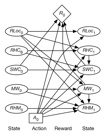
Feature models the robot’s location. The parents of variables are and .
Feature is true when the robot has coffee. The parents of are , , and ; whether the robot has coffee depends on whether it had coffee before, what action it performed, and its location. The probabilities can encode the possibilities that the robot does not succeed in picking up or delivering the coffee, that it drops the coffee, or that someone gives it coffee in some other state (which we may not want to say is impossible).
Variable is true when Sam wants coffee. The parents of include , , , and . You would not expect and to be independent because they both depend on whether or not the coffee was successfully delivered. This could be modeled by having one be a parent of the other.
The two-stage belief network representing how the state variables at time 1 depend on the action and the other state variables is shown in Figure 12.20. This figure also shows the reward as a function of the action, whether Sam stopped wanting coffee, and whether there is mail waiting.
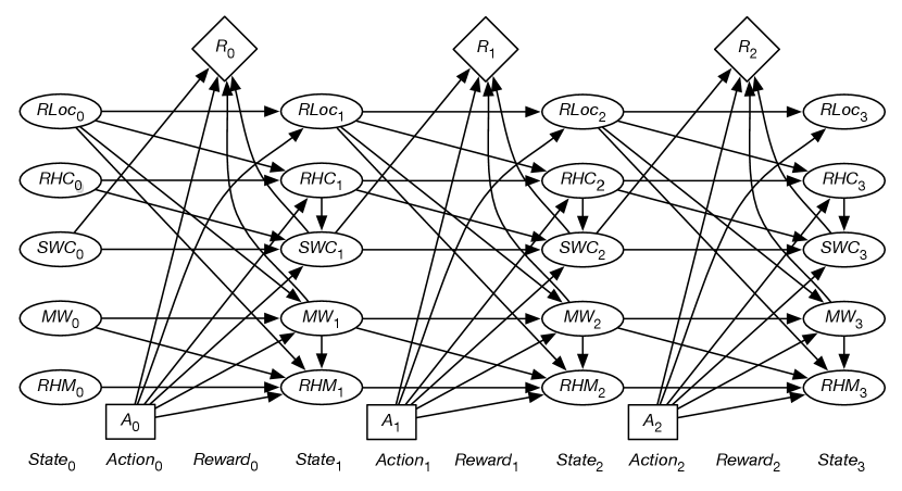
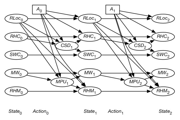
Figure 12.21 shows the unfolded decision network for a horizon of 3.
Example 12.37.
An alternate way to model the dependence between and is to introduce a new variable, , which represents whether coffee was successfully delivered at time . This variable is a parent of both and . Whether Sam wants coffee is a function of whether Sam wanted coffee before and whether coffee was successfully delivered. Whether the robot has coffee depends on the action and the location, to model the robot picking up coffee. Similarly, the dependence between and can be modeled by introducing a variable , which represents whether the mail was successfully picked up. The resulting DDN unfolded to a horizon of 2, but omitting the reward, is shown in Figure 12.22.
If the reward comes only at the end, variable elimination for decision networks, shown in Figure 12.14, can be applied directly. Variable elimination for decision networks corresponds to value iteration. Note that in fully observable decision networks, variable elimination does not require the no-forgetting condition. Once the agent knows the state, all previous decisions are irrelevant. If rewards are accrued at each time step, the algorithm must be augmented to allow for the addition (and discounting) of rewards. See Exercise 12.19.
12.5.5 Partially Observable Decision Processes
A partially observable Markov decision process (POMDP) is a combination of an MDP and a hidden Markov model (HMM). Whereas the state in an MPD is assumed to be fully observable, the environment state in a POMDP is partially observable, which means the agent receives partial and/or noisy observations of the environment before it has to act.
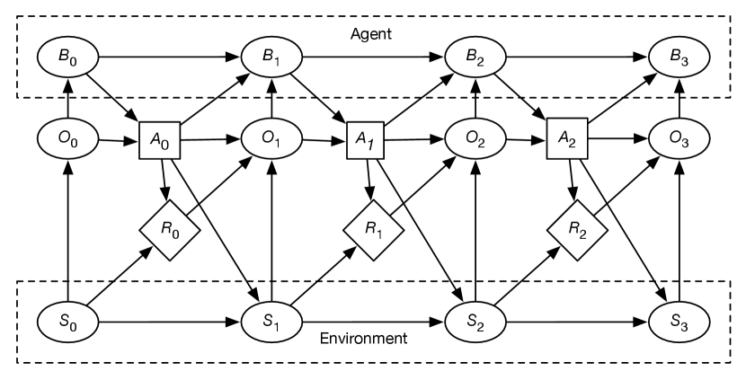
A POMDP can be expressed as the infinite extension of the decision network of Figure 12.23, which explicitly shows the belief state of the agent. The network extends indefinitely to the right.
A POMDP consists of the following variables and factors defining the external behavior of the agent:
-
•
, a set of states of the world
-
•
, a set of actions
-
•
, a set of possible observations
-
•
, the probability distribution of the starting state
-
•
, the dynamics of the environment, is the probability of getting to state by doing action from state
-
•
, the expected reward of starting in state , doing action
-
•
, the probability of observing given the state is , the previous action is , and the reward is .
and are the same as in an MDP. The arc from to means that what the agent observes can depend on the state. The arc from to allows the agent to have actions that don’t affect the environment, but affect its observations, such as paying attention to some part of the environment. The arc from to indicates that the agent’s observation can depend on the reward received; the agent is not assumed to observe the reward directly, as sometimes the rewards are only seen in retrospect. Observing the reward can often provide hints about the state that the agent might not actually be able to observe.
Internally, an agent has
-
•
, the set of possible belief states
-
•
, a belief state transition function, which specifies the agent’s new belief state given the previous belief state , the action the agent did, , and the observation, ; the belief state at stage is .
-
•
, a command function or policy, which specifies a conditional plan defining what the agent will do as a function of the belief state and the observation.
A policy might be stochastic to allow for exploration or to confound other agents. The belief-state transition function is typically deterministic, representing probability distributions, that are updated based on the action and new observations.
Planning in a POMDP involves creating both a belief state transition function and a command function. The variables are special in that the world does not specify the domain or structure of these variables; an agent or its designer gets to choose the structure of a belief state, and how the agent acts based on its belief state, previous action, and latest observations. The belief state encodes all that the agent has remembered about its history.
There are a number of ways to represent a belief state and to find the optimal policy:
-
•
The decision network of Figure 12.23 can be solved using variable elimination for decision networks, shown in Figure 12.14, extended to include discounted rewards. Adding the no-forgetting arcs is equivalent to a belief state being the sequence of observations and actions; is and appended to the sequence . The problem with this approach is that the history is unbounded, and the size of a policy is exponential in the length of the history. This is only practical when the history is short or is deliberately cut short.
-
•
The belief state can be a probability distribution over the states of the environment. Maintaining the belief state is then the problem of filtering in the associated hidden Markov model. The problem with this approach is that, with world states, the set of belief states is an -dimensional real space. The agent then needs to find the optimal function from this multidimensional real space into the actions. The value of a sequence of actions only depends on the world states; as the belief state is a probability distribution over world states, the expected value of a belief state is a linear function of the values of the world states. Not all points in are possible belief states, only those resulting from sequences of observations are possible. Policies can be represented as a decision tree with conditions being (functions of) the observations. The observations dictate which path in the tree the agent will follow. The value function for an agent choosing the best policy for any finite look-ahead is piecewise linear and convex. Although this is simpler than a general function, the number of conditional policies grows like , where is the set of possible observations, and is the stage.
-
•
In general, the belief state can be anything. A belief state can include probability distributions over some of the variables, and remembered observations and actions. The agent can search over the space of controllers for the best controller. Thus, the agent searches over what to remember (the belief state) and what to do based on its belief state. Note that the first two proposals are instances of this approach: the agent’s belief state is all of its history, or the agent’s belief state is a probability distribution over world states, both of which are intractable. Because the general case is unconstrained over what to remember, the search space is enormous.
Artificial Intelligence: Foundations of Computational Agents, Poole
& Mackworth
Copyright © 2023, David L. Poole and Alan K. Mackworth. 
This work is licensed under a Creative Commons Attribution-NonCommercial-NoDerivatives 4.0 International License.