Artificial
Intelligence 3E
foundations of computational agents
14.4 Reasoning with Imperfect Information
In an imperfect-information game, or a partially observable game, an agent does not fully know the state of the world or the agents act simultaneously.
Partial observability for the multiagent case is more complicated than the fully observable multiagent case or the partially observable single-agent case. The following simple examples show some important issues that arise even in the case of two agents, each with a few choices.
Example 14.9.
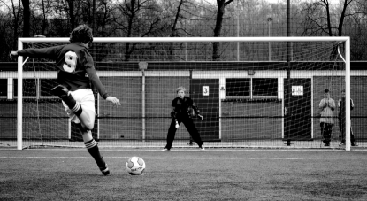
Consider the case of a penalty kick in soccer as depicted in Figure 14.8.
 |
|
||||||||||||||||||||||||
If the kicker kicks to their right and the goalkeeper jumps to their right, the probability of a goal is , and similarly for the other combinations of actions, as given in the figure.
What should the kicker do, given that they want to maximize the probability of a goal and the goalkeeper wants to minimize the probability of a goal? The kicker could think that it is better kicking to their right, because the pair of numbers for their right kick is higher than the pair for the left. The goalkeeper could then think that if the kicker will kick right, they should jump left. However, if the kicker thinks that the goalkeeper will jump left, they should then kick left. But then, the goalkeeper should jump right. Then the kicker should kick right…
Each agent is potentially faced with an infinite regression of reasoning about what the other agent will do. At each stage in their reasoning, the agents reverse their decision. One could imagine cutting this off at some depth; however, the actions then are purely a function of the arbitrary depth. Even worse, if the goalkeeper knew the depth limit of reasoning for the kicker, they could exploit this knowledge to determine what the kicker will do and choose their action appropriately.
An alternative is for the agents to choose actions stochastically. Imagine that the kicker and the goalkeeper each secretly toss a coin to decide what to do. Consider whether the coins should be biased. Suppose that the kicker decides to kick to their right with probability and that the goalkeeper decides to jump to their right with probability . The probability of a goal is then
where the numbers (0.9, 0.3, etc.) come from Figure 14.8.
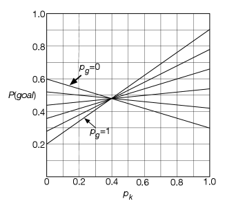
Figure 14.9 shows the probability of a goal as a function of . The different lines correspond to different values of .
There is something special about the value . At this value, the probability of a goal is , independent of the value of . That is, no matter what the goalkeeper does, the kicker expects to get a goal with probability . If the kicker deviates from , they could do better or could do worse, depending on what the goalkeeper does.
The plot for is similar, with all of the lines meeting at . Again, when , the probability of a goal is .
The strategy with and is special in the sense that neither agent can do better by unilaterally deviating from the strategy. However, this does not mean that they cannot do better; if one of the agents deviates from this equilibrium, the other agent could do better by also deviating from the equilibrium. However, this equilibrium is safe for an agent in the sense that, even if the other agent knew the agent’s strategy, the other agent cannot force a worse outcome for the agent. Playing this strategy means that an agent does not have to worry about double-guessing the other agent. In this game, each agent will get the best payoff it could guarantee to obtain.
So let us now extend the definition of a strategy to include randomized strategies.
Consider the normal form of a game where each agent chooses an action simultaneously. Each agent chooses an action without knowing what the other agents choose.
A strategy for an agent is a probability distribution over the actions for this agent. In a pure strategy, one of the probabilities will be 1 and the rest will be 0. Thus, an agent following a pure strategy is acting deterministically. The alternative to a pure strategy is a stochastic strategy, where none of the probabilities are 1, and so more than one action has a non-zero probability. The set of actions with a non-zero probability in a strategy is the support set of the strategy.
A strategy profile is an assignment of a strategy to each agent. If is a strategy profile, let be the strategy of agent in , and let be the strategies of the other agents. Then is . If the strategy profile is made up of pure strategies, it is often called an action profile, because each agent is playing a particular action.
A strategy profile has an expected utility for each agent. Let be the expected utility of strategy profile for agent . The utility of a stochastic strategy profile can be computed by averaging the utilities of the basic actions that make up the profile given the probabilities of the actions.
A best response for an agent to the strategies of the other agents is a strategy that has maximal utility for that agent. That is, is a best response to if, for all other strategies for agent :
A strategy profile is a Nash equilibrium if, for each agent , strategy is a best response to . That is, a Nash equilibrium is a strategy profile such that no agent can do better by unilaterally deviating from that profile.
One of the great results of game theory, proved by Nash [1950], is that every finite game has at least one Nash equilibrium.
Example 14.10.
In Example 14.9, there is a unique Nash equilibrium where and . This has the property that, if the kicker is playing , it does not matter what the goalkeeper does; the goalkeeper will have the same payoff, and so is a best response (as is any other strategy). Similarly, if the goalkeeper is playing , it does not matter what the kicker does; and so every strategy, including , is a best response.
The only reason an agent would consider randomizing between two actions is if the actions have the same expected utility. All probabilistic mixtures of the two actions have the same utility. The reason to choose a particular value for the probability of the mixture is to prevent the other agent from exploiting a deviation.
Games can have multiple Nash equilibria. Consider the following two-agent, two-action game.
Example 14.11.
Suppose there is a resource that two agents may want to fight over. Each agent chooses to act as a hawk or as a dove. Suppose the resource is worth units, where . If both agents act as doves, they share the resource. If one agent acts as a hawk and the other as a dove, the hawk agent gets the resource and the dove agent gets nothing. If they both act like hawks, there is destruction of the resource and the reward to both is , where . This is depicted by the following payoff matrix:
| Agent 2 | |||
|---|---|---|---|
| dove | hawk | ||
| Agent 1 | dove | ||
| hawk | |||
In this matrix, Agent 1 gets to choose the row, Agent 2 gets to choose the column, and the payoff in the cell is a pair consisting of the reward to Agent 1 and the reward to Agent 2. Each agent is trying to maximize its own reward.
In this game there are three Nash equilibria:
-
•
In one equilibrium, Agent 1 acts as a hawk and Agent 2 as a dove. Agent 1 does not want to deviate because then they have to share the resource. Agent 2 does not want to deviate because then there is destruction.
-
•
In the second equilibrium, Agent 1 acts as a dove and Agent 2 as a hawk.
-
•
In the third equilibrium, both agents act stochastically. In this equilibrium, there is some chance of destruction. The probability of acting like a hawk goes up with the value of the resource and goes down as the value of destruction increases. See Exercise 14.3.
In this example, you could imagine each agent doing some posturing to try to indicate what it will do to try to force an equilibrium that is advantageous to it.
Having multiple Nash equilibria does not come from being adversaries, as the following example shows.
Example 14.12.
Suppose there are two people who want to be together. Agent 1 prefers they both go to the football game and Agent 2 prefers they both go shopping. They both would be unhappy if they are not together. Suppose they both have to choose simultaneously what activity to do. This is depicted by the following payoff matrix:
| Agent 2 | |||
|---|---|---|---|
| football | shopping | ||
| Agent 1 | football | ||
| shopping | |||
In this matrix, Agent 1 chooses the row, and Agent 2 chooses the column.
In this game, there are three Nash equilibria. One equilibrium is where they both go shopping, one is where they both go to the football game, and one is a randomized strategy.
This is a coordination problem. Knowing the set of equilibria does not actually tell either agent what to do, because what an agent should do depends on what the other agent will do. In this example, you could imagine conversations to determine which equilibrium they would choose.
Even when there is a unique Nash equilibrium, that Nash equilibrium does not guarantee the maximum payoff to each agent. The following example is a variant of what is known as the prisoner’s dilemma.
Example 14.13.
Imagine you are on a game show with a stranger who you will never see again. You each have the choice of
-
•
taking $100 for yourself, or
-
•
giving $1000 to the other person.
This is depicted as the following payoff matrix:
| Player 2 | |||
|---|---|---|---|
| take | give | ||
| Player 1 | take | ||
| give | |||
No matter what the other agent does, each agent is better off if it takes rather than gives. However, both agents are better off if they both give rather than if they both take.
Thus, there is a unique Nash equilibrium, where both agents take. This strategy profile results in each player receiving $100. The strategy profile where both players give results in each player receiving $1000. However, in this strategy profile, each agent is rewarded for deviating.
There is a large body of research on the prisoner’s dilemma, because it does not seem to be so rational to be greedy, where each agent tries to do the best for itself, resulting in everyone being worse off. One case where giving becomes preferred is when the game is played a number of times. This is known as the sequential prisoner’s dilemma. One strategy for the sequential prisoner’s dilemma is tit-for-tat: each player gives initially, then does the other agent’s previous action at each step. This strategy is a Nash equilibrium as long as there is no last action that both players know about. See Exercise 14.8.
Having multiple Nash equilibria arises not just from partial observability. It is possible to have multiple equilibria with a perfect-information game, and it is even possible to have infinitely many Nash equilibria, as the following example shows.
Example 14.14.
Consider the sharing game of Example 14.2. In this game there are infinitely many Nash equilibria. There is a set of equilibria where Andy shares, and Barb says to sharing for the center choice and can randomize between the other choices, as long as the probability of saying in the left-hand choice is less than or equal to 0.5. In these Nash equilibria, they both get 1. There is another set of Nash equilibria where Andy keeps, and Barb randomizes among her choices, so that the probability of saying in the left branch is greater than or equal to 0.5. In these equilibria, Barb gets 0 and Andy gets some value in the range depending on Barb’s probability. There is a third set of Nash equilibria where Barb has a 0.5 probability of selecting at the leftmost node, selects at the center node, and Andy randomizes between and with any probability.
Suppose the sharing game were modified slightly so that Andy offered a small bribe for Barb to say . This could be done by changing the payoff to be . Andy may think, “Given the choice between getting 0.1 or 0, Barb will choose to get 0.1, so then I should .” But Barb could think, “I should say to 0.1, so that Andy shares and I get 1.” In this example (even ignoring the rightmost branch), there are multiple pure Nash equilibria. One is where Andy keeps and Barb says at the leftmost branch. In this equilibrium, Andy gets 1.9 and Barb gets 0.1. There is another Nash equilibrium where Barb says at the leftmost choice node and at the center branch and Andy chooses . In this equilibrium, they both get 1. It would seem that this is the one preferred by Barb. However, Andy could think that Barb is making an empty threat. If he actually decided to , Barb, acting to maximize her utility, would not actually say .
The backward-induction algorithm only finds one of the equilibria in the modified sharing game of the previous example. It computes a subgame-perfect equilibrium, where it is assumed that the agents choose the action with greatest utility for them at every node where they get to choose. It assumes that agents do not carry out threats that it is not in their interest to carry out at the time. In the modified sharing game of the previous example, it assumes that Barb will say to the small bribe. However, when dealing with real opponents, you should be aware that they may follow through with threats that you may not think rational. Indeed, it might be better for an agent not to (appear to) be rational!
14.4.1 Computing Nash Equilibria
To compute a Nash equilibrium for a game in normal form, there are three steps:
-
1.
Eliminate dominated strategies.
-
2.
Determine the support set, the set of actions which have non-zero probabilities.
-
3.
Determine the probability for the actions in the support set.
It turns out that the second of these is the most difficult.
Eliminating Dominated Strategies
A strategy for agent is dominated by strategy for if, for every action of the other agents, the utility of for agent is lower than the utility of for agent . This is formalized below. Any pure strategy dominated by another strategy can be eliminated from consideration. The dominating strategy could be a randomized strategy. Removing dominated strategies can be done repeatedly.
Example 14.15.
Consider the following payoff matrix, where the first agent chooses the row and the second agent chooses the column. In each cell is a pair of payoffs: the payoff for Agent 1 and the payoff for Agent 2. Agent 1 has actions . Agent 2 has actions .
| Agent 2 | ||||
|---|---|---|---|---|
| Agent 1 | ||||
(Before looking at the solution, try to work out what each agent should do.)
Action can be removed because it is dominated by action : Agent 1 will never do if action is available to it. Notice how the payoff for Agent 1 is greater doing than doing , no matter what the other agent does.
Once action is eliminated, action can be eliminated because it is dominated for Agent 2 by the randomized strategy .
Once and have been eliminated, is dominated by , and so Agent 1 will do action . Given that Agent 1 will do , Agent 2 will do . Thus the unique Nash equilibrium has Agent 1 doing and Agent 2 doing , with a payoff of 3 for Agent 1 and 5 for Agent 2.
Strategy strictly dominates strategy for Agent if, for all action profiles of the other agents:
in which case is strictly dominated by . If is a pure strategy that is strictly dominated by some strategy , then can never be in the support set of any Nash equilibrium. This holds even if is a stochastic strategy. Repeated elimination of strictly dominated strategies gives the same result, regardless of the order in which the strictly dominated strategies are removed.
There are also weaker notions of domination, where the greater than symbol in the preceding formula is replaced by greater than or equal. If the weaker notion of domination is used, there is always a Nash equilibrium with support of the non-dominated strategies. However, some Nash equilibria may be lost. Which equilibria are lost can depend on the order in which the dominated strategies are removed.
Computing Randomized Strategies
An agent will only randomize among actions if the actions all have the same utility to the agent, given the strategies of the other agents. This idea leads to a set of constraints that can be solved to compute a Nash equilibrium. If these constraints can be solved with numbers in the range , and the mixed strategies computed for each agent are not dominated by another strategy for the agent, then this strategy profile is a Nash equilibrium.
Recall that a support set is a set of pure strategies that each have non-zero probability in a Nash equilibrium.
Once dominated strategies have been eliminated, an agent can search over support sets to determine whether the support sets form a Nash equilibrium. Note that, if there are actions available to an agent, there are non-empty subsets, and we have to search over combinations of support sets for the various agents. This is not feasible unless there are only a few non-dominated actions or there are Nash equilibria with small support sets. To find simple (in terms of the number of actions in the support set) equilibria, an agent can search from smaller support sets to larger sets.
Suppose agent is randomizing actions in a Nash equilibrium, each with a non-zero probability. Let be the probability that agent does action . Let be the strategies for the other agents, which is a function of their probabilities. The fact that this is a Nash equilibrium gives the following constraints: , , and, for all
You also require that the utility of doing is not less than the utility of doing an action outside of the support set. Thus, for all :
Example 14.16.
In Example 14.9, suppose the goalkeeper jumps right with probability and the kicker kicks right with probability .
If the goalkeeper jumps right, the probability of a goal is
If the goalkeeper jumps left, the probability of a goal is
The only time the goalkeeper would randomize is if these are equal; that is, if
Solving for gives .
Similarly, for the kicker to randomize, the probability of a goal must be the same whether the kicker kicks left or right:
Solving for gives .
Thus, the only Nash equilibrium has and .
Artificial Intelligence: Foundations of Computational Agents, Poole
& Mackworth
Copyright © 2023, David L. Poole and Alan K. Mackworth. 
This work is licensed under a Creative Commons Attribution-NonCommercial-NoDerivatives 4.0 International License.