12 Planning with Uncertainty 12.2 One-Off Decisions 12.4 The Value of Information and Control

12.3 Sequential Decisions

Generally, agents do not make decisions in the dark without observing something about the world, nor do they make just a single decision. A more typical scenario is that the agent makes an observation, decides on an action, carries out that action, makes observations in the resulting world, then makes another decision conditioned on the observations, and so on. Subsequent actions can depend on what is observed, and what is observed can depend on previous actions. In this scenario, it is often the case that the sole reason for carrying out an action is to provide information for future actions. Actions that are carried out just to acquire information are called information-seeking actions. Such actions are only ever needed in partially observable environments. The formalism does not need to distinguish information-seeking actions from other actions. Typically actions will have both information outcomes as well as effects on the world.

A sequential decision problem models

•

what actions are available to the agent at each stage
•

what information is, or will be, available to the agent when it has to act
•

the effects of the actions, and
•

the desirability of these effects.

Example 12.13.

Consider a simple case of diagnosis where a doctor first chooses some tests and then treats a patient, taking into account the outcome of the tests. The reason the doctor may decide to do a test is so that some information (the test results) will be available at the next stage when treatment may be performed. The test results will be information that is available when the treatment is decided, but not when the test is decided. It is often a good idea to test, even if testing itself may harm the patient.

The actions available are the possible tests and the possible treatments. When the test decision is made, the information available will be the symptoms exhibited by the patient. When the treatment decision is made, the information available will be the patient’s symptoms, what tests were performed, and the test results. The effect of the test is the test result, which depends on what test was performed and what is wrong with the patient. The effect of the treatment is some function of the treatment and what is wrong with the patient. The utility may include, for example, costs of tests and treatments, the pain and inconvenience to the patient in the short term, and the long-term prognosis.

12.3.1 Decision Networks

A decision network (also called an influence diagram) is a graphical representation of a finite sequential decision problem. Decision networks extend belief networks to include decision variables and utility. A decision network extends the single-stage decision network to allow for sequential decisions, and allows both chance nodes and decision nodes to be parents of decision nodes.

In particular, a decision network is a directed acyclic graph (DAG) with chance nodes (drawn as ovals), decision nodes (drawn as rectangles), and a utility node (drawn as a diamond). The meaning of the arcs is as follows.

•

Arcs coming into decision nodes represent the information that will be available when the decision is made.
•

Arcs coming into chance nodes represent probabilistic dependence.
•

Arcs coming into the utility node represent what the utility depends on.

Refer to caption — Figure 12.9: Decision network for decision of whether to take an umbrella

Example 12.14.

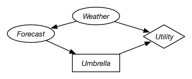
Figure 12.9 shows a simple decision network for a decision of whether the agent should take an umbrella when it goes out. The agent’s utility depends on the weather and whether it takes an umbrella. The agent does not get to observe the weather; it only observes the forecast. The forecast probabilistically depends on the weather.

As part of this network, the designer must specify the domain for each random variable and the domain for each decision variable. Suppose the random variable $W e a t h e r$ has domain $\{norain,rain\}$ , the random variable $F o r e c a s t$ has domain $\{sunny,rainy,cloudy\}$ , and the decision variable $U m b r e l l a$ has domain $\{take\_it,leave\_it\}$ . There is no domain associated with the utility node. The designer also must specify the probability of the random variables given their parents. Suppose $P(Weather)$ is defined by

P(Weather{\,{=}\,}rain)=0.3.

$P(Forecast\mid Weather)$ is given by

$W e a t h e r$	$F o r e c a s t$	Probability
$n o r a i n$	$s u n n y$	0.7
$n o r a i n$	$c l o u d y$	0.2
$n o r a i n$	$r a i n y$	0.1
$r a i n$	$s u n n y$	0.15
$r a i n$	$c l o u d y$	0.25
$r a i n$	$r a i n y$	0.6

Suppose the utility function, $u(Weather,Umbrella)$ , is

$W e a t h e r$	$U m b r e l l a$	$U t i l i t y$
$n o r a i n$	$take\_it$	20
$n o r a i n$	$leave\_it$	100
$r a i n$	$take\_it$	70
$r a i n$	$leave\_it$	0

There is no table specified for the $U m b r e l l a$ decision variable. It is the task of the planner to determine which value of $U m b r e l l a$ to select, as a function of the forecast.

Example 12.15.

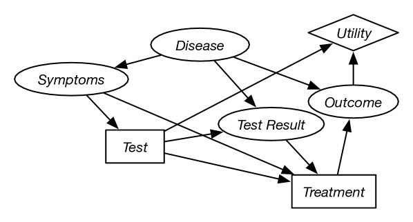
Figure 12.10 shows a decision network that represents the idealized diagnosis scenario of Example 12.13. The symptoms depend on the disease. What test to perform is decided based on the symptoms. The test result depends on the disease and the test performed. The treatment decision is based on the symptoms, the test performed, and the test result. The outcome depends on the disease and the treatment. The utility depends on the costs of the test and on the outcome.

The outcome does not depend on the test, but only on the disease and the treatment, so the test presumably does not have side-effects. The treatment does not directly affect the utility; any cost of the treatment can be incorporated into the outcome. The utility needs to depend on the test unless all tests cost the same amount.

The diagnostic assistant that is deciding on the tests and the treatments never actually finds out what disease the patient has, unless the test result is definitive, which it, typically, is not.

Example 12.16.

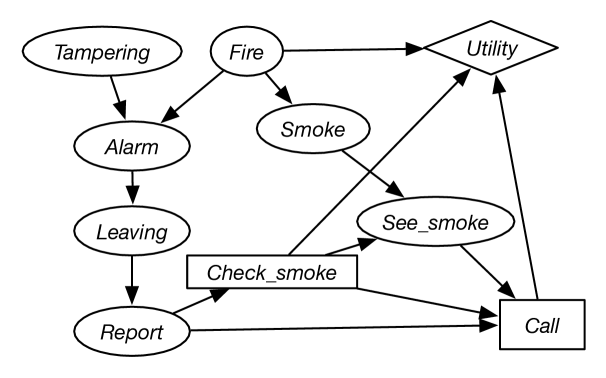
Figure 12.11 gives a decision network that is an extension of the belief network of Figure 9.3. The agent can receive a report of people leaving a building and has to decide whether or not to call the fire department. Before calling, the agent can check for smoke, but this has some cost associated with it. The utility depends on whether it calls, whether there is a fire, and the cost associated with checking for smoke.

In this sequential decision problem, there are two decisions to be made. First, the agent must decide whether to check for smoke. The information that will be available when it makes this decision is whether there is a report of people leaving the building. Second, the agent must decide whether or not to call the fire department. When making this decision, the agent will know whether there was a report, whether it checked for smoke, and whether it can see smoke. Assume that all of the variables are binary.

The information necessary for the decision network includes the conditional probabilities of the belief network and

•

$P(See\_smoke\mid Smoke,Check\_smoke)$ – how seeing smoke depends on whether the agent looks for smoke and whether there is smoke. Assume that the agent has a perfect sensor for smoke. It will see smoke if and only if it looks for smoke and there is smoke. See Exercise 12.9.

•

$u(Check\_smoke,Fire,Call)$ – how the utility depends on whether the agent checks for smoke, whether there is a fire, and whether the fire department is called. Figure 12.12 provides this utility information.

$Check\_smoke$	$F i r e$	$C a l l$	$U t i l i t y$
$y e s$	$t r u e$	$y e s$	$-220$
$y e s$	$t r u e$	$n o$	$-5020$
$y e s$	$f a l s e$	$y e s$	$-220$
$y e s$	$f a l s e$	$n o$	$-20$
$n o$	$t r u e$	$y e s$	$-200$
$n o$	$t r u e$	$n o$	$-5000$
$n o$	$f a l s e$	$y e s$	$-200$
$n o$	$f a l s e$	$n o$	$0$

Figure 12.12: Utility for fire alarm decision network

This utility function expresses the cost structure that calling has a cost of 200, checking has a cost of 20, but not calling when there is a fire has a cost of 5000. The utility is the negative of the cost.

A no-forgetting agent is an agent whose decisions are totally ordered in time, and the agent remembers its previous decisions and any information that was available to a previous decision.

A no-forgetting decision network is a decision network in which the decision nodes are totally ordered and, if decision node $D_{i}$ is before $D_{j}$ in the total ordering, then $D_{i}$ is a parent of $D_{j}$ , and any parent of $D_{i}$ is also a parent of $D_{j}$ .

Thus, any information available to $D_{i}$ is available to any subsequent decision, and the action chosen for decision $D_{i}$ is part of the information available for subsequent decisions. The no-forgetting condition is sufficient to make sure that the following definitions make sense and that the following algorithms work.

12.3.2 Policies

A policy specifies what the agent should do under all contingencies. A policy consists of a decision function for each decision variable. A decision function for a decision variable is a function that specifies a value for the decision variable for each assignment of values to its parents. Thus, a policy specifies, for each decision variable, what the agent will do for each of the possible observations.

Example 12.17.

In Example 12.14, some of the policies are:

•

Always bring the umbrella.
•

Bring the umbrella only if the forecast is “rainy.”
•

Bring the umbrella only if the forecast is “sunny.”

There are eight different policies, because there are three possible forecasts and there are two choices for each forecast.

Example 12.18.

In Example 12.16, a policy specifies a decision function for $Check\_smoke$ and a decision function for $C a l l$ . Some of the policies are:

•

Never check for smoke, and call only if there is a report.
•

Always check for smoke, and call only if it sees smoke.
•

Check for smoke if there is a report, and call only if there is a report and it sees smoke.
•

Check for smoke if there is no report, and call when it does not see smoke.
•

Always check for smoke and never call.

There are four decision functions for $Check\_smoke$ . There are $2^{8}$ decision functions for $C a l l$ ; for each of the eight assignments of values to the parents of $C a l l$ , the agent can choose to call or not. Thus there are $4*2^{8}=1024$ different policies.

Expected Utility of a Policy

Each policy has an expected utility for an agent that follows the policy. A rational agent should adopt the policy that maximizes its expected utility.

A possible world specifies a value for each random variable and each decision variable. A possible world $\omega$ satisfies policy $\pi$ if for every decision variable $D$ , $D(\omega)$ has the value specified by the policy given the values of the parents of $D$ in the possible world.

A possible world corresponds to a complete history and specifies the values of all random and decision variables, including all observed variables. Possible world $\omega$ satisfies policy $\pi$ if $\omega$ is one possible unfolding of history given that the agent follows policy $\pi$ .

The expected utility of policy $\pi$ is

{\mathcal{E}}(u\mid\pi)=\sum_{\omega\mbox{\scriptsize{} satisfies }\pi}u(% \omega)*P(\omega)

where $P(\omega)$ , the probability of world $\omega$ , is the product of the probabilities of the values of the chance nodes given their parents’ values in $\omega$ , and $u(\omega)$ is the value of the utility $u$ in world $\omega$ .

Example 12.19.

Consider Example 12.14, let $\pi_{1}$ be the policy to take the umbrella if the forecast is cloudy and to leave it at home otherwise. The worlds that satisfy this policy are:

$W e a t h e r$	$F o r e c a s t$	$U m b r e l l a$
$n o r a i n$	$s u n n y$	$leave\_it$
$n o r a i n$	$c l o u d y$	$take\_it$
$n o r a i n$	$r a i n y$	$leave\_it$
$r a i n$	$s u n n y$	$leave\_it$
$r a i n$	$c l o u d y$	$take\_it$
$r a i n$	$r a i n y$	$leave\_it$

Notice how the value for the decision variable is the one chosen by the policy. It only depends on the forecast.

The expected utility of this policy is obtained by averaging the utility over the worlds that satisfy this policy:

	$\displaystyle{\mathcal{E}}(u\mid\pi_{1})=\mbox{}$	$\displaystyle P(norain)P(sunny\mid norain)u(norain,leave\_it)$
		$\displaystyle\mbox{}+P(norain)P(cloudy\mid norain)u(norain,take\_it)$
		$\displaystyle\mbox{}+P(norain)P(rainy\mid norain)u(norain,leave\_it)$
		$\displaystyle\mbox{}+P(rain)P(sunny\mid rain)u(rain,leave\_it)$
		$\displaystyle\mbox{}+P(rain)P(cloudy\mid rain)u(rain,take\_it)$
		$\displaystyle\mbox{}+P(rain)P(rainy\mid rain)u(rain,leave\_it)$

where $n o r a i n$ means $Weather=norain$ , $s u n n y$ means $Forecast=sunny$ , and similarly for the other values.

An optimal policy is a policy $\pi^{*}$ such that ${\mathcal{E}}(u\mid\pi^{*})\geq{\mathcal{E}}(u\mid\pi)$ for all policies $\pi$ . That is, an optimal policy is a policy whose expected utility is maximal over all policies.

Suppose a binary decision node has $n$ binary parents. There are $2^{n}$ different assignments of values to the parents and, consequently, there are $2^{2^{n}}$ different possible decision functions for this decision node. The number of policies is the product of the number of decision functions for each of the decision variables. Even small examples can have a huge number of policies. An algorithm that simply enumerates the policies looking for the best one will be very inefficient.

12.3.3 Optimizing Decision Networks using Search

The recursive conditioning algorithm for belief networks can be extended to decision networks as follows:

•

It takes a context, a set of factors for the conditional distributions of the random variables and the utility, and a set of decision variables.
•

It returns a value for the optimal policy given the context and optimal decision functions for the decision variables for that context. The decision functions are represented as a set of $\left<context,d{\,{=}\,}v\right>$ pairs, which means the optimal decision has decision variable $d$ taking value $v$ in $c o n t e x t$ .
•

The splitting order has the parents of each decision node come before the node, and these are the only nodes before the decision node. In particular, it cannot select a variable to split on that is not a parent of all remaining decision nodes. Thus, it is only applicable to no-forgetting decision networks. If it were to split on a variable $X$ that is not a parent of a decision variable $d$ , it can make a different choice of a value for $d$ depending on the value of $X$ , which cannot be implemented by an agent that does not know the value of $X$ when it has to do $d$ .
•

The utility node does not need to be treated differently from the factors defining probabilities; the utility just provides a number that is multiplied by the probabilities.
•

To split on a decision node, the algorithm chooses a value that maximizes the values returned for each assignment of a value for that node.

1: procedure DN_dfs(

{Con}

{Fs}

{Ds}

)

2: #

{Con}

:contest,

{Fs}

: set of factors,

{Ds}

: set of decision variables

3: # Returns a value, and set of

\left<context,d{\,{=}\,}v\right>

pairs

4: if

{Fs}=\{\}

then

5: return

(1,\{\})

6: else if

f\in{Fs}

can be evaluated in

{Con}

then

(v,p)\;{:}{=}\;\mbox{}DN\_dfs({Con},{Fs}\setminus\{f\},{Ds})

8: return

(eval(f,{Con})*v,p)

9: else if

C o n

assigns all parents of decision node

d\in{Ds}

then

10:

max\_value\;{:}{=}\;\mbox{}-\infty;~{}~{}opt\_decn\;{:}{=}\;\mbox{}\bot

11: for

v a l

domain(d)

12:

(v,p)\;{:}{=}\;\mbox{}DN\_dfs(Con\cup\{d{\,{=}\,}val\},Fs,{Ds}\setminus\{d\})

13: if

v>max\_value

then

14:

max\_value\;{:}{=}\;\mbox{}v;~{}~{}opt\_decn\;{:}{=}\;\mbox{}\{\left<Con,d{\,{% =}\,}val\right>\}\cup p

15: return

(max\_value,opt\_decn)

16: else

17: select variable

v a r

vars(Fs)\setminus vars({Con})

that is a parent of all

d\in{Ds}

18:

sum:=0;policy=\{\}

19: for

v a l

domain(var)

20:

(v,p):=DN\_dfs(Con\cup\{var{\,{=}\,}val\},Fs,{Ds})

21:

sum:=sum+v;~{}policy\;{:}{=}\;\mbox{}policy\cup p

22: return

(sum,policy)

Figure 12.13: Search-based optimization algorithm for decision networks

Figure 12.13 extends the naive search algorithm of Figure 9.9 to solve decision networks. It is easiest to think of this algorithm as computing a sum over products, choosing the maximum value when there is a choice. The value returned by the recursive call is a mix of the probability and utility.

Example 12.20.

Consider Example 12.16. The algorithm first splits on $R e p o r t$ as it is a parent of all decision nodes. Consider the $f a l s e$ branch. It then calls $DN\_dfs$ with context $\{Report{\,{=}\,}false\}$ , and the decision variable $Check\_smoke$ is split. The recursive call will determine whether it is better to check when the report is false. It then splits on $See\_smoke$ and then $C a l l$ . The other factors can be eliminated in any order.

The call to $DN\_dfs$ with context $\{Report{\,{=}\,}false\}$ returns the pair

\left<P(Report{\,{=}\,}false)*utility(\pi),\pi\right>

where $\pi$ is the optimal policy when $Report{\,{=}\,}false$ .

Table 12.1 shows what factors can be evaluated for one variable ordering.

Variable	Factor(s) Evaluated
$R e p o r t$	–
$Check\_smoke$	–
$See\_Smoke$	–
$C a l l$	–
$T a m p e r i n g$	$P(Tampering)$
$F i r e$	$P(Fire)$ , $Utility(Fire,See\_smoke,Call)$
$S m o k e$	$P(Fire\mid Smoke)$ , $P(See\_smoke\mid Smoke)$
$A l a r m$	$P(Alarm\mid Tampering,Fire)$
$L e a v i n g$	$P(Leaving\mid Alarm)$ , $P(Report\mid Leaving)$

Table 12.1: Variables split on and factors evaluated for Example 12.20

It is difficult to interpret the numbers being returned by the recursive calls. Some are just products of probability (recursive calls after the $U t i l i t y$ factor is evaluated), and some are a mix of probability and utility. The easiest way to think about this is that the algorithm is computing the sum of a product of numbers, maximizing for a choice at the decision nodes.

The algorithm of Figure 12.13 does not exploit the independence of graphical structure, but all of the enhancements of recursive conditioning, namely recognizing disconnected components and judicious caching can be incorporated unchanged.

12.3.4 Variable Elimination for Decision Networks

Variable elimination can be adapted to find an optimal policy. The idea is first to consider the last decision, find an optimal decision for each value of its parents, and produce a factor of these maximum values. This results in a new decision network, with one less decision, that can be solved recursively.

1: procedure VE_DN(

D N

2: Inputs

D N

a decision network

4: Output

5: An optimal policy and its expected utility

6: Local

D F s

: a set of decision functions, initially empty

F s

: a set of factors

9: Remove all variables that are not ancestors of the utility node

10: Create a factor in

F s

for each conditional probability

11: Create a factor in

F s

for the utility

12: while there are decision nodes remaining do

13: Sum out each random variable that is not a parent of a decision node

14: Let

D

be the last decision remaining

15: # $D$ is only in a factor $F(D,V_{1},\dots,V_{k})$ where $V_{1},\dots,V_{k}$ are parents of $D$

16: Add

\max_{D}F

F s

17: Add

\arg\max_{D}F

D F s

18: Sum out all remaining random variables

19: Return

D F s

and the product of remaining factors

Figure 12.14: Variable elimination for decision networks

Figure 12.14 shows how to use variable elimination for decision networks. Essentially, it computes the expected utility of an optimal decision. It eliminates the random variables that are not parents of a decision node by summing them out according to some elimination ordering. The ordering of the random variables being eliminated does not affect correctness and so it can be chosen for efficiency.

After eliminating all of the random variables that are not parents of a decision node, in a no-forgetting decision network, there must be one decision variable $D$ that is in a factor $F$ where all of the variables, other than $D$ , in $F$ are parents of $D$ . This decision $D$ is the last decision in the ordering of decisions.

To eliminate that decision node, $VE\_DN$ chooses the values for the decision that result in the maximum utility. This maximization creates a new factor on the remaining variables and a decision function for the decision variable being eliminated. This decision function created by maximizing is one of the decision functions in an optimal policy.

Example 12.21.

In Example 12.14, there are three initial factors representing $P(Weather)$ , $P(Forecast\mid Weather)$ , and $u(Weather,Umbrella)$ . First, it eliminates $W e a t h e r$ by multiplying all three factors and summing out $W e a t h e r$ , giving a factor on $F o r e c a s t$ and $U m b r e l l a$ , shown on left of Table 12.2.

$F o r e c a s t$	$U m b r e l l a$	Value
$s u n n y$	$take\_it$	12.95
$s u n n y$	$leave\_it$	49.0
$c l o u d y$	$take\_it$	8.05
$c l o u d y$	$leave\_it$	14.0
$r a i n y$	$take\_it$	14.0
$r a i n y$	$leave\_it$	7.0

$F o r e c a s t$	$U m b r e l l a$
$s u n n y$	$leave\_it$
$c l o u d y$	$leave\_it$
$r a i n y$	$take\_it$

$F o r e c a s t$	Value
$s u n n y$	49.0
$c l o u d y$	14.0
$r a i n y$	14.0

Table 12.2: Factors and decision functions created in Example 12.21

To maximize over $U m b r e l l a$ , for each value of $F o r e c a s t$ , $VE\_DN$ selects the value of $U m b r e l l a$ that maximizes the value of the factor. For example, when the forecast is $s u n n y$ , the agent should leave the umbrella at home for a value of 49.0. The resulting decision function is shown in Table 12.2 (center), and the resulting factor is shown in Table 12.2 (right).

It now sums out $F o r e c a s t$ from this factor, which gives the value 77.0. This is the expected value of the optimal policy.

Example 12.22.

Consider Example 12.16. The initial factors are shown in Table 12.3.

Initial factors:

\begin{array}[]{ll}Meaning&Factor\\ \hline\cr P(Tampering)&f_{0}(Tampering)\\ P(Fire)&f_{1}(Fire)\\ P(Alarm\mid Tampering,Fire)&f_{2}(Tampering,Fire,Alarm)\\ P(Smoke\mid Fire)&f_{3}(Fire,Smoke)\\ P(Leaving\mid Alarm)&f_{4}(Alarm,Leaving)\\ P(Report\mid Leaving)&f_{5}(Leaving,Report)\\ P(See\_smoke\mid Check\_smoke,Smoke){}{}{}{}&f_{6}(Smoke,See\_smoke,Check\_% smoke)\\ u(Fire,Check\_smoke,Call)&f_{7}(Fire,Check\_smoke,Call)\end{array}

The factors that are removed and created for one elimination ordering:

Variable	How	Removed	Factor Created
$T a m p e r i n g$	sum	$f_{0}$ , $f_{2}$	$f_{8}(Fire,Alarm)$
$F i r e$	sum	$f_{1}$ , $f_{8}$ , $f_{3}$ , $f_{7}$	$f_{9}(Alarm,Smoke,Check\_Smoke,Call)$
$A l a r m$	sum	$f_{4}$ , $f_{9}$	$f_{10}(Smoke,Check\_Smoke,Call,Leaving)$
$S m o k e$	sum	$f_{10}$ , $f_{6}$	$f_{11}(Check\_Smoke,Leaving,See\_Smoke,Call)$
$L e a v i n g$	sum	$f_{5}$ , $f_{11}$	$f_{12}(Report,See\_Smoke,Check\_Smoke,Call)$
$C a l l$	max	$f_{12}$	$f_{13}(Check\_Smoke,See\_Smoke,Report)$
$See\_smoke$	sum	$f_{13}$	$f_{14}(Check\_Smoke,Report)$
$Check\_smoke$	max	$f_{14}$	$f_{15}(Report)$
$R e p o r t$	sum	$f_{15}$	$f_{16}$

Table 12.3: Initial and created factors in Example 12.22

The expected utility is the product of the probability and the utility, as long as the appropriate actions are chosen.

Table 12.3 (bottom) shows the factors that are removed and created for one elimination ordering. The random variables that are not parents of a decision node are summed out first.

The factor $f_{16}$ is a number that is the expected utility of the optimal policy.

The following gives more detail of one of the factors. After summing out $T a m p e r i n g$ , $F i r e$ , $A l a r m$ , $S m o k e$ , and $L e a v i n g$ , there is a single factor, $f_{12}$ , part of which (to two decimal places) is

$R e p o r t$	$See\_smoke$	$Check\_smoke$	$C a l l$	Value
$t r u e$	$t r u e$	$y e s$	$y e s$	$-1.33$
$t r u e$	$t r u e$	$y e s$	$n o$	$-29.30$
$t r u e$	$t r u e$	$n o$	$y e s$	0
$t r u e$	$t r u e$	$n o$	$n o$	0
$t r u e$	$f a l s e$	$y e s$	$y e s$	$-4.86$
$t r u e$	$f a l s e$	$y e s$	$n o$	$-3.68$
…	…	…	…	…

From this factor, an optimal decision function can be created for $C a l l$ by selecting a value for $C a l l$ that maximizes $V a l u e$ for each assignment to $R e p o r t$ , $See\_smoke$ , and $Check\_smoke$ .

Consider the case when $Report{\,{=}\,}true$ , $See\_smoke{\,{=}\,}true$ , and $Check\_smoke{\,{=}\,}yes$ . The maximum of $-1.33$ and $-29.3$ is $-1.33$ , so for this case, the optimal action is $Call{\,{=}\,}yes$ with value $-1.33$ . This maximization is repeated for the other values of $R e p o r t$ , $See\_smoke$ , and $Check\_smoke$ .

An optimal decision function for $C a l l$ is

$R e p o r t$	$See\_smoke$	$Check\_smoke$	$C a l l$
$t r u e$	$t r u e$	$y e s$	$y e s$
$t r u e$	$t r u e$	$n o$	$y e s$
$t r u e$	$f a l s e$	$y e s$	$n o$
…	…	…	…

The value for $C a l l$ when $Report{\,{=}\,}true$ , $See\_smoke{\,{=}\,}true$ , and $Check\_smoke{\,{=}\,}no$ is arbitrary. It does not matter what the agent plans to do in this situation, because the situation never arises. The algorithm does not need to treat this as a special case.

The factor resulting from maximizing $C a l l$ contains the maximum values for each combination of $R e p o r t$ , $See\_smoke$ , and $Check\_smoke$ :

$R e p o r t$	$See\_smoke$	$Check\_smoke$	Value
$t r u e$	$t r u e$	$y e s$	$-1.33$
$t r u e$	$t r u e$	$n o$	0
$t r u e$	$f a l s e$	$y e s$	$-3.68$
…	…	…	…

Summing out $See\_smoke$ gives the factor

$R e p o r t$	$Check\_smoke$	Value
$t r u e$	$y e s$	$-5.01$
$t r u e$	$n o$	$-5.65$
$f a l s e$	$y e s$	$-23.77$
$f a l s e$	$n o$	$-17.58$

Maximizing $Check\_smoke$ for each value of $R e p o r t$ gives the decision function

$R e p o r t$	$Check\_smoke$
$t r u e$	$y e s$
$f a l s e$	$n o$

and the factor

$R e p o r t$	Value
$t r u e$	$-5.01$
$f a l s e$	$-17.58$

Summing out $R e p o r t$ gives the expected utility of $-22.60$ (taking into account rounding errors).

Thus, the policy returned can be seen as the rules

check\_smoke\leftarrow\mbox{}report.

call\leftarrow\mbox{}see\_smoke.

call\leftarrow\mbox{}report\wedge\mbox{}\neg check\_smoke\wedge\mbox{}\neg see% \_smoke.

The last of these rules is never used because the agent following the optimal policy does check for smoke if there is a report. It remains in the policy because $VE\_DN$ has not determined an optimal policy for $Check\_smoke$ when it is optimizing $C a l l$ .

Note also that, in this case, even though checking for smoke has an immediate negative reward, checking for smoke is worthwhile because the information obtained is valuable.

The following example shows how the factor containing a decision variable can contain a subset of its parents when the VE algorithm optimizes the decision.

Example 12.23.

Consider Example 12.14, but with an extra arc from $W e a t h e r$ to $U m b r e l l a$ . That is, the agent gets to observe both the weather and the forecast. In this case, there are no random variables to sum out, and the factor that contains the decision node and a subset of its parents is the original utility factor. It can then maximize $U m b r e l l a$ , giving the decision function and the factor:

$W e a t h e r$	$U m b r e l l a$
$n o r a i n$	$leave\_it$
$r a i n$	$take\_it$

$W e a t h e r$	$V a l u e$
$n o r a i n$	100
$r a i n$	70

Note that the forecast is irrelevant to the decision. Knowing the forecast does not give the agent any useful information. Summing out $F o r e c a s t$ gives a factor where all of the values are 1.

Summing out $W e a t h e r$ , where $P(Weather{\,{=}\,}norain)=0.7$ , gives the expected utility $0.7*100+0.3*70=91$ .

Variable elimination for decision networks of Figure 12.14 has similar complexity to the combination of depth-first search of Figure 12.13 with recursive conditioning. They are carrying out the same computations on a different order. In particular, the values stored in the cache of recursive conditioning are the same as the values in the factors of variable elimination. Recursive conditioning allows for the exploitation of various representations of conditional probability, but storing the values in a cache is less efficient than storing the values using a tabular representation. When the networks are infinite, as below, the more sophisticated algorithms are usually based on one or the other.

	$\displaystyle{\mathcal{E}}(u\mid\pi_{1})=\mbox{}$	$\displaystyle P(norain)P(sunny\mid norain)u(norain,leave\_it)$
		$\displaystyle\mbox{}+P(norain)P(cloudy\mid norain)u(norain,take\_it)$
		$\displaystyle\mbox{}+P(norain)P(rainy\mid norain)u(norain,leave\_it)$
		$\displaystyle\mbox{}+P(rain)P(sunny\mid rain)u(rain,leave\_it)$
		$\displaystyle\mbox{}+P(rain)P(cloudy\mid rain)u(rain,take\_it)$
		$\displaystyle\mbox{}+P(rain)P(rainy\mid rain)u(rain,leave\_it)$

Artificial Intelligence 3E

12.3 Sequential Decisions

Example 12.13.

12.3.1 Decision Networks

Example 12.14.

Example 12.15.

Example 12.16.

12.3.2 Policies

Example 12.17.

Example 12.18.

Expected Utility of a Policy

Example 12.19.

12.3.3 Optimizing Decision Networks using Search

Example 12.20.

12.3.4 Variable Elimination for Decision Networks

Example 12.21.

Example 12.22.

Example 12.23.

Artificial
Intelligence 3E