12 Planning with Uncertainty 12.1 Preferences and Utility 12.3 Sequential Decisions

12.2 One-Off Decisions

Basic decision theory applied to intelligent agents relies on the following assumptions:

•

Agents know what actions they can carry out.
•

The effect of each action can be described as a probability distribution over outcomes.
•

An agent’s preferences are expressed by utilities of outcomes.

It is a consequence of Proposition 12.3 that, if agents only act for one step, a rational agent should choose an action with the highest expected utility.

Example 12.7.

Consider the problem of the delivery robot in which there is uncertainty in the outcome of its actions. In particular, consider the problem of going from position $o109$ in Figure 3.1 to the $m a i l$ position, where there is a chance that the robot will slip off course and fall down the stairs. Suppose the robot can get pads that will not change the probability of an accident but will make an accident less severe. Unfortunately, the pads add extra weight. The robot could also go the long way around, which would reduce the probability of an accident but make the trip much slower.

Thus, the robot has to decide whether to wear the pads and which way to go (the long way or the short way). What is not under its direct control is whether there is an accident, although this probability can be reduced by going the long way around. For each combination of the agent’s choices and whether there is an accident, there is an outcome ranging from severe damage to arriving quickly without the extra weight of the pads.

In one-off decision making, a decision variable is used to model an agent’s choice. A decision variable is like a random variable, but it does not have an associated probability distribution. Instead, an agent gets to choose a value for a decision variable. A possible world specifies values for both random and decision variables. Each possible world has an associated utility. For each combination of values to decision variables, there is a probability distribution over the random variables. That is, for each assignment of a value to each decision variable, the measures of the worlds that satisfy that assignment sum to $1$ .

Refer to caption — Figure 12.6: A decision tree for the delivery robot. Square boxes represent decisions that the robot can make. Circles represent random variables that the robot cannot observe before making its decision

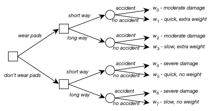
Figure 12.6 shows a decision tree that depicts the different choices available to the agent and the outcomes of those choices. To read the decision tree, start at the root (on the left in this figure). For the decision nodes, shown as squares, the agent gets to choose which branch to take. For each random node, shown as a circle, the agent does not get to choose which branch will be taken; rather, there is a probability distribution over the branches from that node. Each leaf corresponds to a world, which is the outcome if the path to that leaf is followed.

Example 12.8.

In Example 12.7 there are two decision variables, one corresponding to the decision of whether the robot wears pads and one to the decision of which way to go. There is one random variable, whether there is an accident or not. Eight possible worlds correspond to the eight paths in the decision tree of Figure 12.6.

What the agent should do depends on how important it is to arrive quickly, how much the pads’ weight matters, how much it is worth to reduce the damage from severe to moderate, and the likelihood of an accident.

The proof of Proposition 12.3 specifies how to measure the desirability of the outcomes. Suppose we decide to have utilities in the range [0,100]. First, choose the best outcome, which would be $w_{5}$ , and give it a utility of $100$ . The worst outcome is $w_{6}$ , so assign it a utility of $0$ . For each of the other worlds, consider the lottery between $w_{6}$ and $w_{5}$ . For example, $w_{0}$ may have a utility of 35, meaning the agent is indifferent between $w_{0}$ and $[0.35:w_{5},0.65:w_{6}]$ , which is slightly better than $w_{2}$ , which may have a utility of 30. $w_{1}$ may have a utility of 95, because it is only slightly worse than $w_{5}$ .

Example 12.9.

In medical diagnosis, decision variables correspond to various treatments and tests. The utility may depend on the costs of tests and treatment and whether the patient gets better, stays sick, or dies, and whether they have short-term or chronic pain. The outcomes for the patient depend on the treatment the patient receives, the patient’s physiology, and the details of the disease, which may not be known with certainty.

The same approach holds for diagnosis of artifacts such as airplanes; engineers test components and fix them. In airplanes, you may hope that the utility function is to minimize accidents (maximize safety), but the utility incorporated into such decision making is often to maximize profit for a company and accidents are simply costs taken into account.

In a one-off decision, the agent chooses a value for each decision variable simultaneously. This can be modeled by treating all the decision variables as a single composite decision variable, $D$ . The domain of this decision variable is the cross product of the domains of the individual decision variables.

Each world $\omega$ specifies an assignment of a value to the decision variable $D$ and an assignment of a value to each random variable. Each world has a utility, given by the variable $u$ .

A single decision is an assignment of a value to the decision variable. The expected utility of single decision $D=d_{i}$ is ${\mathcal{E}}(u\mid D=d_{i})$ , the expected value of the utility conditioned on the value of the decision. This is the average utility of the worlds, where the worlds are weighted according to their probability:

{\mathcal{E}}(u\mid D=d_{i})=\sum_{\omega:D(\omega)=d_{i}}u(\omega)*{P(\omega)}

where $D(\omega)$ is the value of variable $D$ in world $\omega$ , $u(\omega)$ is the value of utility in $\omega$ , and $P(\omega)$ is the probability of world $\omega$ .

An optimal single decision is the decision whose expected utility is maximal. That is, $D=d_{max}$ is an optimal decision if

{\mathcal{E}}(u\mid D=d_{max})=\max_{d_{i}\in domain(D)}{\mathcal{E}}(u\mid D=% d_{i})

where $domain(D)$ is the domain of decision variable $D$ . Thus

d_{max}=\arg\max_{d_{i}\in domain(D)}{\mathcal{E}}(u\mid D=d_{i}).

Example 12.10.

The delivery robot problem of Example 12.7 is a single decision problem where the robot has to decide on the values for the variables $Wear\_pads$ and $Which\_way$ . The single decision is the complex decision variable $\left<Wear\_pads,Which\_way\right>$ . Each assignment of a value to each decision variable has an expected value. For example, the expected utility of $Wear\_pads=true\wedge Which\_way=short$ is given by

{\mathcal{E}}(u\mid wear\_pads\wedge Which\_way=short)

\mbox{}=P(accident\mid wear\_pads\wedge Which\_way=short)*u(w_{0})

\mbox{}+(1-P(accident\mid wear\_pads\wedge Which\_way=short))*u(w_{1})

where $u(w_{i})$ is the value of the utility in worlds $w_{i}$ , the worlds $w_{0}$ and $w_{1}$ are as in Figure 12.6, and $wear\_pads$ means $Wear\_pads=true$ .

12.2.1 Single-Stage Decision Networks

A decision tree is a state-based representation where each path from a root to a leaf corresponds to a state. It is, however, often more natural and more efficient to represent and reason directly in terms of features, represented as variables.

A single-stage decision network is an extension of a belief network with three kinds of nodes:

•

Decision nodes, drawn as rectangles, represent decision variables. The agent gets to choose a value for each decision variable. Where there are multiple decision variables, we assume there is a total ordering of the decision nodes, and the decision nodes before a decision node $D$ in the total ordering are the parents of $D$ .
•

Chance nodes, drawn as ovals, represent random variables. These are the same as the nodes in a belief network. Each chance node has an associated domain and a conditional probability of the variable, given its parents. As in a belief network, the parents of a chance node represent conditional dependence: a variable is independent of its non-descendants, given its parents. In a decision network, both chance nodes and decision nodes can be parents of a chance node.
•

A single utility node, drawn as a diamond, represents the utility. The parents of the utility node are the variables on which the utility depends. Both chance nodes and decision nodes can be parents of the utility node.

Each chance variable and each decision variable has a domain. There is no domain for the utility node. Whereas the chance nodes represent random variables and the decision nodes represent decision variables, there is no utility variable.

Associated with a decision network is a conditional probability for each chance node given its parents (as in a belief network) and a utility as a function of the utility node’s parents. In the specification of the network, there are no functions associated with a decision (although the algorithm will construct a function).

$Which\_way$	$A c c i d e n t$	Value
$s h o r t$	$t r u e$	0.2
$s h o r t$	$f a l s e$	0.8
$l o n g$	$t r u e$	0.01
$l o n g$	$f a l s e$	0.99

$Wear\_pads$	$Which\_way$	$A c c i d e n t$	Utility
$t r u e$	$s h o r t$	$t r u e$	35
$t r u e$	$s h o r t$	$f a l s e$	95
$t r u e$	$l o n g$	$t r u e$	30
$t r u e$	$l o n g$	$f a l s e$	75
$f a l s e$	$s h o r t$	$t r u e$	3
$f a l s e$	$s h o r t$	$f a l s e$	100
$f a l s e$	$l o n g$	$t r u e$	0
$f a l s e$	$l o n g$	$f a l s e$	80

Example 12.11.

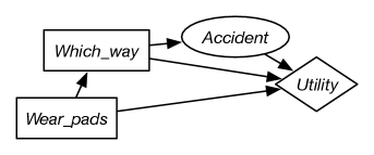
Figure 12.7 gives a decision network representation of Example 12.7. There are two decisions to be made: which way to go and whether to wear padding. Whether the agent has an accident only depends on which way they go. The utility depends on all three variables.

This network requires two factors: a factor representing the conditional probability, $P(Accident\mid Which\_way)$ , and a factor representing the utility as a function of $Which\_way$ , $A c c i d e n t$ , and $Wear\_pads$ . Tables for these factors are shown in Figure 12.7.

A policy for a single-stage decision network is an assignment of a value to each decision variable. Each policy has an expected utility. An optimal policy is a policy whose expected utility is maximal. That is, it is a policy such that no other policy has a higher expected utility. The value of a decision network is the expected utility of an optimal policy for the network.

1: procedure VE_SSDN(

D N

)

2: Inputs

D N

a single-stage decision network

4: Output

5: An optimal policy and the expected utility of that policy.

6: Prune all nodes that are not ancestors of the utility node.

7: Sum out all chance nodes.

8: – at this stage there is a single factor

F

that was derived from utility

9: Let

v

be the maximum value in

F

10: Let

d

be an assignment that gives the maximum value

11: return

d, v

Figure 12.8: Variable elimination for a single-stage decision network

Figure 12.8 shows how variable elimination is used to find an optimal policy in a single-stage decision network. After pruning irrelevant nodes and summing out all random variables, there will be a single factor that represents the expected utility for each combination of decision variables. This factor does not have to be a factor on all of the decision variables; however, those decision variables that are not included are not relevant to the decision.

Example 12.12.

Consider running ${VE\_SSDN}$ on the decision network of Figure 12.7. No nodes are able to be pruned, so it sums out the only random variable, $A c c i d e n t$ . To do this, it multiplies both factors because they both contain $A c c i d e n t$ , and sums out $A c c i d e n t$ , giving the following factor:

$Wear\_pads$	$Which\_way$	Value
$t r u e$	$s h o r t$	$0.235+0.895=83$
$t r u e$	$l o n g$	$0.0130+0.9975=74.55$
$f a l s e$	$s h o r t$	$0.23+0.8100=80.6$
$f a l s e$	$l o n g$	$0.010+0.9980=79.2$

Thus, the policy with the maximum value – the optimal policy – is to take the short way and wear pads, with an expected utility of 83.

Artificial Intelligence 3E