Artificial
Intelligence 2E
foundations of computational agents
The third edition of Artificial Intelligence: foundations of computational agents, Cambridge University Press, 2023 is now available (including full text).
9.5 Decision Processes
Dimensions: flat, states, infinite horizon, fully observable, stochastic, utility, non-learning, single agent, offline, perfect rationality
The decision networks of the previous section were for finite-stage, partially observable domains. In this section, we consider indefinite horizon and infinite horizon problems.
Often an agent must reason about an ongoing process or it does not know how many actions it will be required to do. These are called infinite horizon problems when the process may go on forever or indefinite horizon problems when the agent will eventually stop, but it does not know when it will stop.
For ongoing processes, it may not make sense to consider only the utility at the end, because the agent may never get to the end. Instead, an agent can receive a sequence of rewards. These rewards incorporate the action costs in addition to any prizes or penalties that may be awarded. Negative rewards are called punishments. Indefinite horizon problems can be modeled using a stopping state. A stopping state or absorbing state is a state in which all actions have no effect; that is, when the agent is in that state, all actions immediately return to that state with a zero reward. Goal achievement can be modeled by having a reward for entering such a stopping state.
A Markov decision process can be seen as a Markov chain augmented with actions and rewards or as a decision network extended in time. At each stage, the agent decides which action to perform; the reward and the resulting state depend on both the previous state and the action performed.
We only consider stationary models where the state transitions and the rewards do not depend on the time.
A Markov decision process or an MDP consists of
-
•
, a set of states of the world
-
•
, a set of actions
-
•
, which specifies the dynamics. This is written as , the probability of the agent transitioning into state given that the agent is in state and does action . Thus,
-
•
, where , the reward function, gives the expected immediate reward from doing action and transitioning to state from state . Sometimes it is convenient to use , the expected value of doing in state , which is .
A finite part of a Markov decision process can be depicted using a decision network as in Figure 9.14.
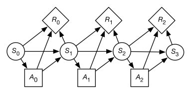
Example 9.27.
Suppose Sam wanted to make an informed decision about whether to party or relax over the weekend. Sam prefers to party, but is worried about getting sick. Such a problem can be modeled as an MDP with two states, and , and two actions, and . Thus
Based on experience, Sam estimate that the dynamics is given by
| Probability of | ||
|---|---|---|
| 0.95 | ||
| 0.7 | ||
| 0.5 | ||
| 0.1 |
So, if Sam is healthy and parties, there is a 30% chance of becoming sick. If Sam is healthy and relaxes, Sam will more likely remain healthy. If Sam is sick and relaxes, there is a 50% chance of getting better. If Sam is sick and parties, there is only a 10% chance of becoming healthy.
Sam estimates the (immediate) rewards to be:
| Reward | ||
|---|---|---|
| 7 | ||
| 10 | ||
| 0 | ||
| 2 |
Thus, Sam always enjoys partying more than relaxing. However, Sam feels much better overall when healthy, and partying results in being sick more than relaxing does.
The problem is to determine what Sam should do each weekend.
Example 9.28.
A grid world is an idealization of a robot in an environment. At each time, the robot is at some location and can move to neighboring locations, collecting rewards and punishments. Suppose that the actions are stochastic, so that there is a probability distribution over the resulting states given the action and the state.
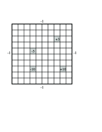
Figure 9.15 shows a grid world, where the robot can choose one of four actions: up, down, left, or right. If the agent carries out one of these actions, it has a chance of going one step in the desired direction and a chance of going one step in any of the other three directions. If it bumps into the outside wall (i.e., the location computed is outside the grid), there is a penalty of 1 (i.e., a reward of ) and the agent does not actually move. There are four rewarding states (apart from the walls), one worth (at position ; 9 across and 8 down), one worth (at position ), one worth (at position ), and one worth (at position ). In each of these states, the agent gets the reward after it carries out an action in that state, not when it enters the state. When the agent reaches one of the states with positive reward (either or ), no matter what action it performs, at the next step it is flung, at random, to one of the four corners of the grid world.
Note that, in this example, the reward is a function of both the initial state and the final state. The agent bumped into the wall, and so received a reward of , if and only if the agent remains is the same state. Knowing just the initial state and the action, or just the final state and the action, does not provide enough information to infer the reward.
As with decision networks, the designer also has to consider what information is available to the agent when it decides what to do. There are two common variations:
-
•
In a fully observable Markov decision process (MDP), the agent gets to observe the current state when deciding what to do.
-
•
A partially observable Markov decision process (POMDP) is a combination of an MDP and a hidden Markov model. At each time, the agent gets to make some (ambiguous and possibly noisy) observations that depend on the state. The agent only has access to the history of rewards, observations and previous actions when making a decision. It cannot directly observe the current state.
Rewards
To decide what to do, the agent compares different sequences of rewards. The most common way to do this is to convert a sequence of rewards into a number called the value, the cumulative reward or the return. To do this, the agent combines an immediate reward with other rewards in the future. Suppose the agent receives the sequence of rewards:
Three common reward criteria are used to combine rewards into a value :
- Total reward
-
. In this case, the value is the sum of all of the rewards. This works when you can guarantee that the sum is finite; but if the sum is infinite, it does not give any opportunity to compare which sequence of rewards is preferable. For example, a sequence of $1 rewards has the same total as a sequence of $100 rewards (both are infinite). One case where the total reward is finite is when there are stopping states and the agent always has a non-zero probability of eventually entering a stopping state.
- Average reward
-
. In this case, the agent’s value is the average of its rewards, averaged over for each time period. As long as the rewards are finite, this value will also be finite. However, whenever the total reward is finite, the average reward is zero, and so the average reward will fail to allow the agent to choose among different actions that each have a zero average reward. Under this criterion, the only thing that matters is where the agent ends up. Any finite sequence of bad actions does not affect the limit. For example, receiving $1,000,000 followed by rewards of $1 has the same average reward as receiving $0 followed by rewards of $1 (they both have an average reward of $1).
- Discounted reward
-
, where , the discount factor, is a number in the range . Under this criterion, future rewards are worth less than the current reward. If was 1, this would be the same as the total reward. When , the agent ignores all future rewards. Having guarantees that, whenever the rewards are finite, the total value will also be finite.
The discounted reward can be rewritten as
Suppose is the reward accumulated from time :
To understand the properties of , suppose , then . Solving for gives . Thus, with the discounted reward, the value of all of the future is at most times as much as the maximum reward and at least times as much as the minimum reward. Therefore, the eternity of time from now only has a finite value compared with the immediate reward, unlike the average reward, in which the immediate reward is dominated by the cumulative reward for the eternity of time.
In economics, is related to the interest rate: getting now is equivalent to getting in one year, where is the interest rate. You could also see the discount rate as the probability that the agent survives; can be seen as the probability that the agent keeps going.
The rest of this chapter considers discounted rewards. The discounted reward is referred to as the value.