9.5.4 Dynamic Decision Networks

Dimensions: flat, features, infinite horizon, fully observable, stochastic, utility, non-learning, single agent, offline, perfect rationality

A Markov decision process is a state-based representation. Just as in classical planning, where reasoning in terms of features can allow for more straightforward representations and more efficient algorithms, planning under uncertainty can also take advantage of reasoning in term of features. This forms the basis for decision-theoretic planning.

A dynamic decision network (DDN) can be seen in a number of different ways:

•

a factored representation of MDPs, where the states are described in terms of features
•

an extension of decision networks to allow repeated structure for indefinite or infinite horizon problems
•

an extension of dynamic belief networks to include actions and rewards
•

an extension of the feature-based representation of actions or the CSP representation of planning to allow for rewards and for uncertainty in the effect of actions.

A dynamic decision network consists of

•

a set of state features
•

a set of possible actions
•
a two-stage decision network with chance nodes $F_{0}$ and $F_{1}$ for each feature $F$ (for the features at time 0 and time 1, respectively) and decision node $A_{0}$ , such that
- –
  
  the domain of $A_{0}$ is the set of all actions
- –
  
  the parents of $A_{0}$ are the set of time 0 features (these arcs are often not shown explicitly)
- –
  
  the parents of time 0 features do not include $A_{0}$ or time 1 features, but can include other time 0 features as long as the resulting network is acyclic
- –
  
  the parents of time 1 features can contain $A_{0}$ and other time 0 or time 1 features as long as the graph is acyclic
- –
  
  there are probability distributions for $P(F_{0}\mid parents(F_{0}))$ and $P(F_{1}\mid parents(F_{1}))$ for each feature $F$
- –
  
  the reward function depends on any subset of the action and the features at times 0 or 1.

As in a dynamic belief network, a dynamic decision network can be unfolded into a decision network by replicating the features and the action for each subsequent time. For a time horizon of $n$ , there is a variable $F_{i}$ for each feature $F$ and for each time $i$ for $0\leq i\leq n$ . For a time horizon of $n$ , there is a variable $A_{i}$ for each time $i$ for $0\leq i<n$ . The horizon, $n$ , can be unbounded, which allows us to model processes that do not halt.

Thus, if there are $k$ features for a time horizon of $n$ there are $k*(n+1)$ chance nodes (each representing a random variable) and $k$ decision nodes in the unfolded network.

The parents of $A_{i}$ are random variables $F_{i}$ (so that the agent can observe the state). Each $F_{i+1}$ depends on the action $A_{i}$ and the features at time $i$ and $i+1$ in the same way, with the same conditional probabilities, as $F_{1}$ depends the action $A_{0}$ and the features at time $0$ and $1$ . The $F_{0}$ variables modeled directly in the two-stage decision network.

Example 9.34.

Example 6.1 models a robot that can deliver coffee and mail in a simple environment with four locations. Consider representing a stochastic version of Example 6.1 as a dynamic decision network. We use the same features as in that example.

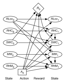
Figure 9.19: Two-stage dynamic decision network

Feature $R L o c$ models the robot’s location. The parents of variables $RLoc_{1}$ are $Rloc_{0}$ and $A$ .

Feature $R H C$ is true when the robot has coffee. The parents of $RHC_{1}$ are $RHC_{0}$ , $A_{0}$ , and $RLoc_{0}$ ; whether the robot has coffee depends on whether it had coffee before, what action it performed, and its location. The probabilities can encode the possibilities that the robot does not succeed in picking up or delivering the coffee, that it drops the coffee, or that someone gives it coffee in some other state (which we may not want to say is impossible).

Variable $S W C$ is true when Sam wants coffee. The parents of $SWC_{1}$ include $SWC_{0}$ , $RHC_{0}$ , $A_{0}$ , and $RLoc_{0}$ . You would not expect $RHC_{1}$ and $SWC_{1}$ to be independent because they both depend on whether or not the coffee was successfully delivered. This could be modeled by having one be a parent of the other.

The two-stage belief network representing how the state variables at time 1 depend on the action and the other state variables is shown in Figure 9.19. This figure also shows the reward as a function of the action, whether Sam stopped wanting coffee, and whether there is mail waiting.

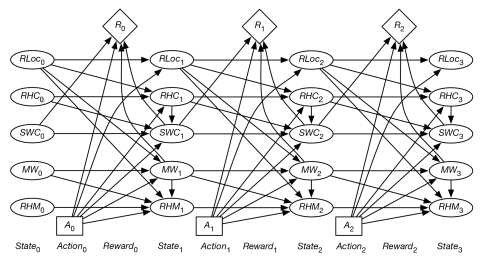
Figure 9.20 shows the unfolded decision network for a horizon of 3.

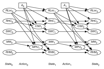
Figure 9.20: Dynamic decision network unfolded for a horizon of 3

Example 9.35.

An alternate way to model the dependence between $RHC_{1}$ and $SWC_{1}$ is to introduce a new variable, $CSD_{1}$ , which represents whether coffee was successfully delivered at time $1$ . This variable is a parent of both $RHC_{1}$ and $SWC_{1}$ . Whether Sam wants coffee is a function of whether Sam wanted coffee before and whether coffee was successfully delivered. Whether the robot has coffee depends on the action and the location, to model the robot picking up coffee. Similarly, the dependence between $MW_{1}$ and $RHM_{1}$ can be modeled by introducing a variable $MPU_{1}$ , which represents whether the mail was successfully picked up. The resulting DDN unfolded to a horizon of 2, but omitting the reward, is shown in Figure 9.21.

Figure 9.21: Dynamic decision network with intermediate variables for a horizon of 2, omitting the reward nodes

If the reward comes only at the end, variable elimination for decision networks, shown in Figure 9.13, can be applied directly. Variable elimination for decision networks corresponds to value iteration. Note that in fully observable decision networks variable elimination does not require the no-forgetting condition. Once the agent knows the state, all previous decisions are irrelevant. If rewards are accrued at each time step, the algorithm must be augmented to allow for the addition (and discounting) of rewards. See Exercise 18.

Artificial Intelligence 2E

9.5.4 Dynamic Decision Networks

Example 9.34.

Example 9.35.

Artificial
Intelligence 2E