8.5 Sequential Probability Models 8.5.1 Markov Chains 8.5.3 Algorithms for Monitoring and Smoothing

The third edition of Artificial Intelligence: foundations of computational agents, Cambridge University Press, 2023 is now available (including full text).

8.5.2 Hidden Markov Models

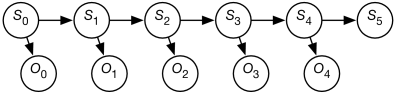
A hidden Markov model (HMM) is an augmentation of a Markov chain to include observations. A hidden Markov model includes the state transition of the Markov chain, and adds to it observations at each time that depend on the state at the time. These observations can be partial in that different states map to the same observation and noisy in that the same state stochastically maps to different observations at different times.

The assumptions behind an HMM are:

•

The state at time $t+1$ only directly depends on the state at time $t$ for $t\geq 0$ , as in the Markov chain.
•

The observation at time $t$ only directly depends on the state at time $t$ .

The observations are modeled using the variable $O_{t}$ for each time $t$ whose domain is the set of possible observations. The belief network representation of an HMM is depicted in Figure 8.12. Although the belief network is shown for five stages, it extends indefinitely.

Figure 8.12: A hidden Markov model as a belief network

A stationary HMM includes the following probability distributions:

•

$P(S_{0})$ specifies initial conditions
•

$P(S_{t+1}\mid S_{t})$ specifies the dynamics
•

$P(O_{t}\mid S_{t})$ specifies the sensor model.

Example 8.29.

Suppose you want to keep track of an animal in a triangular enclosure using sound. You have three microphones that provide unreliable (noisy) binary information at each time step. The animal is either near one of the 3 vertices of the triangle or close to the middle of the triangle. The state has domain $\{m,c_{1},c_{2},c_{3}\}$ where $m$ means the animal is in the middle and $c_{i}$ means the animal is in corner $i$ .

The dynamics of the world is a model of how the state at one time depends on the previous time. If the animal is in a corner it stays in the same corner with probability 0.8, goes to the middle with probability 0.1 or goes to one of the other corners with probability 0.05 each. If it is in the middle, it stays in the middle with probability 0.7, otherwise it moves to one of the corners, each with probability 0.1.

The sensor model specifies the probability of detection by each microphone given the state. If the animal is in a corner, it will be detected by the microphone at that corner with probability 0.6, and will be independently detected by each of the other microphones with a probability of 0.1. If the animal is in the middle, it will be detected by each microphone with a probability of 0.4.

Initially the animal is in one of the four states, with equal probability.

There are a number of tasks that are common for HMMs.

The problem of filtering or belief-state monitoring is to determine the current state based on the current and previous observations, namely to determine

P(S_{i}\mid O_{0},\dots,O_{i}).

All state and observation variables after $S_{i}$ are irrelevant because they are not observed and can be ignored when this conditional distribution is computed.

Example 8.30.

Consider filtering for Example 8.29.

The following table gives the observations for each time, and the resulting state distribution. There are no observations at time 0.

	Observation			Posterior State Distribution
Time	Mic#1	Mic#2	Mic#3	$P(m)$	$P(c_{1})$	$P(c_{2})$	$P(c_{3})$
0	–	–	–	0.25	0.25	0.25	0.25
1	0	1	1	0.46	0.019	0.26	0.26
2	1	0	1	0.64	0.084	0.019	0.26

Thus, even with only two time steps of noisy observations from initial ignorance, it is very sure that the animal is not at corner 1 or corner 2. It is most likely that the animal is in the middle.

Note that the posterior at any time only depended on the observations up to that time. Filtering does not take into account future observations that provide more information about the initial state.

The problem of smoothing is to determine a state based on past and future observations. Suppose an agent has observed up to time $k$ and wants to determine the state at time $i$ for $i<k$ ; the smoothing problem is to determine

P(S_{i}\mid O_{0},\dots,O_{k}).

All of the variables $S_{i}$ and $V_{i}$ for $i>k$ can be ignored.

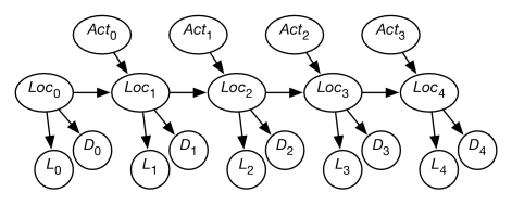
Localization

Suppose a robot wants to determine its location based on its history of actions and its sensor readings. This is the problem of localization.

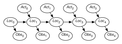
Figure 8.13 shows a belief-network representation of the localization problem. There is a variable $Loc_{i}$ for each time $i$ , which represents the robot’s location at time $i$ . There is a variable $Obs_{i}$ for each time $i$ , which represents the robot’s observation made at time $i$ . For each time $i$ , there is a variable $Act_{i}$ that represents the robot’s action at time $i$ . In this section, assume that the robot’s actions are observed. (The case in which the robot chooses its actions is discussed in Chapter 9).

This model assumes the following dynamics: At time $i$ , the robot is at location $Loc_{i}$ , it observes $Obs_{i}$ , then it acts, it observes its action $Act_{i}$ , and time progresses to time $i+1$ , where it is at location $Loc_{i+1}$ . Its observation at time $t$ only depends on the state at time $t$ . The robot’s location at time $t+1$ depends on its location at time $t$ and its action at time $t$ . Its location at time $t+1$ is conditionally independent of previous locations, previous observations, and previous actions, given its location at time $t$ and its action at time $t$ .

The localization problem is to determine the robot’s location as a function of its observation history:

P(Loc_{t}\mid Obs_{0},Act_{0},Obs_{1},Act_{1},\dots,Act_{t-1},Obs_{t}).

Example 8.31.

Consider the domain depicted in Figure 8.14.

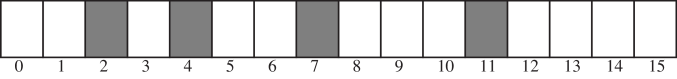
There is a circular corridor, with 16 locations numbered 0 to 15. The robot is at one of these locations at each time. This is modeled with, for every time $i$ , a variable $Loc_{i}$ with domain $\{0,1,\dots,15\}$ .

•

There are doors at positions 2, 4, 7, and 11 and no doors at other locations.
•

The robot has a sensor that noisily senses whether or not it is in front of a door. This is modeled with a variable $Obs_{i}$ for each time $i$ , with domain $\{door,nodoor\}$ . Assume the following conditional probabilities:

$\displaystyle{P(Obs_{t}{=}door\mid atDoor_{t})=0.8}$

$\displaystyle{P(Obs_{t}{=}door\mid notAtDoor_{t})=0.1}$

where $atDoor_{t}$ is true when the robot is at states 2, 4, 7, or 11 at time $t$ , and $notAtDoor_{t}$ is true when the robot is at the other states.

Thus, the observation is partial in that many states give the same observation and it is noisy in the following way: in 20% of the cases in which the robot is at a door, the sensor falsely gives a negative reading. In 10% of the cases where the robot is not at a door, the sensor records that there is a door.

•

The robot can, at each time, move left, move right, or stay still. Assume that the stay still action is deterministic, but the dynamics of the moving actions are stochastic. Just because the robot carries out the $g o R i g h t$ action does not mean that it actually goes one step to the right – it is possible that it stays still, goes two steps right, or even ends up at some arbitrary location (e.g., if someone picks up the robot and moves it). Assume the following dynamics, for each location $L$ :

	$\displaystyle{P(Loc_{t+1}{=}L\mid Act_{t}{=}goRight\wedge Loc_{t}{=}L)=0.1}$
	$\displaystyle{P(Loc_{t+1}{=}L+1\mid Act_{t}{=}goRight\wedge Loc_{t}{=}L)=0.8}$
	$\displaystyle{P(Loc_{t+1}{=}L+2\mid Act_{t}{=}goRight\wedge Loc_{t}{=}L)=0.074}$
	$\displaystyle{P(Loc_{t+1}{=}L^{\prime}\mid Act_{t}{=}goRight\wedge Loc_{t}{=}L% )=0.002\mbox{ for any other location $L^{\prime}$.}}$

All location arithmetic is modulo 16. The action $g o L e f t$ works the same way but to the left.

The robot starts at an unknown location and must determine its location.

It may seem as though the domain is too ambiguous, the sensors are too noisy, and the dynamics is too stochastic to do anything. However, it is possible to compute the probability of the robot’s current location given its history of actions and observations.

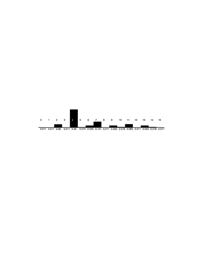
Figure 8.15: A distribution over locations. The locations are numbered from 0 to 15. The number at the bottom gives the posterior probability that the robot is at the location after the particular sequence of actions and observations given in Example 8.31. The height of the bar is proportional to the posterior probability.

Figure 8.15 gives the robot’s probability distribution over its locations, assuming it starts with no knowledge of where it is and experiences the following observations: observe door, go right, observe no door, go right, and then observe door. Location 4 is the most likely current location, with posterior probability of 0.42. That is, in terms of the network of Figure 8.13:

	$\displaystyle P(Loc_{2}=4\mid$	$\displaystyle Obs_{0}=door,Act_{0}=goRight,Obs_{1}=nodoor,$
		$\displaystyle Act_{1}=goRight,Obs_{2}=door)=0.42$

Location 7 is the second most likely current location, with posterior probability of 0.141. Locations 0, 1, 3, 8, 12, and 15 are the least likely current locations, with posterior probability of 0.011.

You can see how well this works for other sequences of observations by using the applet at the book website.

Example 8.32.

Let us augment Example 8.31 with another sensor. Suppose that, in addition to a door sensor, there is also a light sensor. The light sensor and the door sensor are conditionally independent given the state. Suppose the light sensor is not very informative; it only gives yes-or-no information about whether it detects any light, and this is very noisy, and depends on the location.

Figure 8.16: Localization with multiple sensors

This is modeled in Figure 8.16 using the following variables:

•

$Loc_{t}$ is the robot’s location at time $t$
•

$Act_{t}$ is the robot’s action at time $t$
•

$D_{t}$ is the door sensor value at time $t$
•

$L_{t}$ is the light sensor value at time $t$ .

Conditioning on both $L_{i}$ and $D_{i}$ lets it combine information from the light sensor and the door sensor. This is an instance of sensor fusion. It is not necessary to define any new mechanisms for sensor fusion given the belief-network model; standard probabilistic inference combines the information from both sensors.

	$\displaystyle{P(Obs_{t}{=}door\mid atDoor_{t})=0.8}$
	$\displaystyle{P(Obs_{t}{=}door\mid notAtDoor_{t})=0.1}$

Artificial Intelligence 2E