11 Causality 11.2 Missing Data 11.4 Instrumental Variables

11.3 Inferring Causality

You cannot determine the effect of intervention from observational data. However, you can infer causality if you are prepared to make assumptions. A problem with inferring causality is that there can be confounders, other variables correlated with the variables of interest. A confounder between $X$ and $Y$ is a variable $Z$ such that $P(Y\mid X,do(Z))\neq P(Y\mid X)$ and $P(X\mid do(Z))\neq P(X)$ . A confounder can account for the correlation between $X$ and $Y$ by being a common cause of both.

Example 11.7.

Consider the effect of a drug on a disease. The effect of the drug cannot be determined by considering the correlation between taking the drug and the outcome. The reason is that the drug and the outcome can be correlated for other reasons than just the effect of the drug. For example, the severity of a disease and the gender of the patient may be correlated with both, and so potential confounders. If the drug is only given to the sickest people, the drug may be positively correlated with a poor outcome, even though the drug might work very well – it makes each patient less sick than they would have been if they were not given the drug.

The story of how the variables interact could be represented by the network of Figure 11.7. In this figure, the variable $D r u g$ could represent whether the patient was given the drug or not. Whether a patient is given a drug depends on the severity of the disease (variable $S e v e r i t y$ ) and the gender of the person (variable $G e n d e r$ ). You might not be sure whether $G e n d e r$ is a confounder, but because there is a possibility, it can be included to be safe.

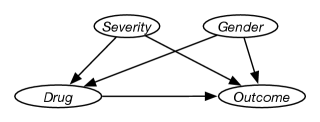
Refer to caption — Figure 11.7: Measuring the effectiveness of a drug

From observational data, $P(outcome\mid drug)$ can be determined, but to determine whether a drug is useful requires $P(outcome\mid do(drug))$ , which is potentially different because of the confounders. The important part of the network of Figure 11.7 are the missing nodes and arcs; this assumes that there are no other confounders.

In a randomized controlled trial one variable (e.g., a drug) is given to patients at random, selected using a random number generator, independently of its parents (e.g., independently of how severe the disease is). In a causal network, this is modeled by removing the arcs into that variable, as it is assumed that the random number generator is not correlated with other variables. This then allows us to determine the effect of making the variable true with all confounders removed.

11.3.1 Backdoor Criterion

If one is prepared to commit to a model, in particular to identify all possible confounders, it is possible to determine causal knowledge from observational data. This is appropriate when you identify all confounders and enough of them are observable.

Example 11.8.

In Example 11.7, there are three reasons why the drug and outcome are correlated. One is the direct effect of the drug on the outcome. The others are due to the confounders of the severity of the disease and the gender of the patient. The aim to measure the direct effect. If the severity and gender are the only confounders, you can adjust for them by considering the effect of the drug on the outcome for each severity and gender separately, and weighting the outcome appropriately:

	$\displaystyle P(Outcome\mid do(Drug))$
	$\displaystyle\mbox{}=\sum_{Severity}\sum_{Gender}$	$\displaystyle P(Severity)*P(Gender)$
		$\displaystyle*P(Outcome\mid do(Drug),Severity,Gender)$
	$\displaystyle\mbox{}=\sum_{Severity}\sum_{Gender}$	$\displaystyle P(Severity)*P(Gender)$
		$\displaystyle*P(Outcome\mid Drug,Severity,Gender).$

The last step follows because $D r u g, S e v e r i t y, G e n d e r$ are all the parents of $O u t c o m e$ , for which, because of the assumption of a causal network, observing and doing have the same effect. These can all be judged without acting.

This analysis relies on the assumptions that severity and gender are the only confounders and both are observable.

The previous example is a specific instance of the backdoor criterion. A set of variables $Z$ satisfies the backdoor criterion for $X$ and $Y$ with respect to directed acyclic graph $G$ if

•

$Z$ can be observed
•

no node in $Z$ is a descendant of $X$ , and
•

$Z$ blocks every path between $X$ and $Y$ that contains an arrow into $X$ .

If $Z$ satisfies the backdoor criterion, then

P(Y\mid do(X))=\sum_{Z}P(Y\mid X,Z)*P(Z).

The aim is to find an observable set of variables $Z$ which blocks all spurious paths from $X$ to $Y$ , leaves all directed paths from $X$ to $Y$ , and doesn’t create any new spurious paths. If $Z$ is observable, the above formula can be estimated from observational data.

It is often challenging, or even impossible, to find a $Z$ that is observable. For example, even though “drug prone” in Example 11.2 blocks all paths in Figure 11.2, because it cannot be measured, it is not useful.

11.3.2 Do-calculus

The do-calculus tells us how probability expressions involving the do-operator can be simplified. It is defined in terms of the following three rules:

•

If $Z$ blocks all of the paths from $W$ to $Y$ in the graph obtained after removing all of the arcs into $X$ :

$P(Y\mid do(X),Z,W)=P(Y\mid do(X),Z).$

This rule lets us remove observations from a conditional probability. This is effectively d-separation in the manipulated graph.
•

If $Z$ satisfies the backdoor criterion, for $X$ and $Y$ :

$P(Y\mid do(X),Z)=P(Y\mid X,Z).$

This rule lets us convert an intervention into an observation.
•

If there are no directed paths from $X$ to $Y$ , or from $Y$ to $X$ :

$P(Y\mid do(X))=P(Y).$

This only can be used when there are no observations, and tells us that the only effects of an intervention are on the descendants of the intervened variable.

These three rules are complete in the sense that all cases where interventions can be reduced to observations follow from applications of these rules.

11.3.3 Front-Door Criterion

Sometimes the backdoor criterion is not applicable because the confounding variables are not observable. One case where it is still possible to derive the effect of an action is when there is an intermediate, mediating variable or variables between the intervention variable and the effect, and where the mediating variable is not affected by the confounding variables, given the intervention variable. This case is covered in the front-door criterion.

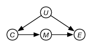
Consider the generic network of Figure 11.8, where the aim is to predict $P(E\mid do(C))$ , where the confounders $U$ are unobserved and the intermediate mediating variable $M$ is independent of $U$ given $C$ . This pattern can be created by collecting all confounders into $U$ , and all mediating variables into $M$ , and marginalizing other variables to fit the pattern.

The backdoor criterion is not applicable here, because $U$ is not observed. When $M$ is observed and is independent of $U$ given $C$ , the do-calculus can be used to infer the effect on $E$ of intervening on $C$ .

Let’s first introduce $M$ and marginalize it out, as in belief network inference:

$\displaystyle P(E\mid do(C))$	$\displaystyle=\sum_{M}P(E\mid do(C),M)*P(M\mid do(C))$
	$\displaystyle=\sum_{M}P(E\mid do(C),do(M))*P(M\mid do(C))$	(11.1)
	$\displaystyle=\sum_{M}P(E\mid do(C),do(M))*P(M\mid C)$	(11.2)
	$\displaystyle=\sum_{M}P(E\mid do(M))*P(M\mid C).$	(11.3)

Step (11.1) follows using the second rule of the do-calculus because $C$ blocks the backdoor between $M$ and $E$ . Step (11.2) uses the second rule of the do-calculus as $\{\}$ satisfies the backdoor criterion between $C$ and $M$ ; there are no backdoors between $C$ and $M$ , given nothing is observed. Step (11.3) uses the third rule of the do-calculus as there are no causal paths from $C$ to $E$ in the graph obtained by removing the arcs into $M$ (which is the effect of $do(M)$ ).

The intervention on $C$ does not affect $P(E\mid do(M))$ . This conditional probability can be computed by introducing $C$ and marginalizing it from the network of Figure 11.8. The $C$ is not intervened on, so let’s give it a new name, $C^{\prime}$ :

\displaystyle P(E\mid do(M))

\displaystyle=\sum_{C^{\prime}}P(E\mid do(M),C^{\prime})*P(C^{\prime}\mid do(M% )).

As $C^{\prime}$ closes the backdoor between $M$ and $E$ , by the second rule, and there are no backdoors between $M$ and $C$ :

	$\displaystyle P(E\mid do(M))$	$\displaystyle=\sum_{C^{\prime}}P(E\mid M,C^{\prime})*P(C^{\prime}\mid do(M))$
		$\displaystyle=\sum_{C^{\prime}}P(E\mid M,C^{\prime})*P(C^{\prime}).$

Thus, $P(E\mid do(C))$ reduces to observable quantities only:

\displaystyle P(E\mid do(C))

\displaystyle=\sum_{M}P(M\mid C)*\sum_{C^{\prime}}P(E\mid M,C^{\prime})*P(C^{% \prime}).

Thus the intervention on $M$ can be inferred from observable data only as long as $C$ is observable and the mediating variable $M$ is observable and independent of all confounders given $C$ .

One of the lessons from this is that it is possible to make causal conclusions from observational data and assumptions on causal mechanisms. Indeed, it is not possible to make causal conclusions without assumptions on causal mechanisms. Even randomized trials require the assumption that the randomizing mechanism is independent of the effects.

11.3.4 Simpson’s Paradox

Simpson’s paradox occurs when considering subpopulations gives different conclusions than considering the population as a whole. This is a case where different conclusions are drawn from the same data, depending on an underlying causal model.

Example 11.9.

Consider the following (fictional) dataset of 1000 students, 500 of whom were using a particular method for learning a concept (the treatment variable $T$ ), and whether they were judged to have understood the concept (evaluation $E$ ) for two subpopulations (one with $C{\,{=}\,}true$ and one with $C{\,{=}\,}false$ ):

$C$	$T$	$E{\,{=}\,}true$	$E{\,{=}\,}false$	Rate
$t r u e$	$t r u e$	90	10	$90/(90+10)=90\%$
$t r u e$	$f a l s e$	290	110	$290/(290+110)=72.5\%$
$f a l s e$	$t r u e$	110	290	$110/(110+290)=27.5\%$
$f a l s e$	$f a l s e$	10	90	$10/(10+90)=10\%$

where the integers are counts, and the rate is the proportion that understood ( $E{\,{=}\,}true$ ). For example, there were 90 students with $C{\,{=}\,}true$ , $T{\,{=}\,}true$ , and $E{\,{=}\,}true$ , and 10 students with $C{\,{=}\,}true$ , $T{\,{=}\,}true$ , and $E{\,{=}\,}false$ , and so 90% of the students with $C{\,{=}\,}true$ , $T{\,{=}\,}true$ have $E{\,{=}\,}true$ .

For both subpopulations, the understanding rate for those who used the method is better than for those who didn’t use the method. So it looks like the method works.

Combining the subpopulations gives

$T$	$E{\,{=}\,}true$	$E{\,{=}\,}false$	Rate
$t r u e$	200	300	$200/(200+300)=40\%$
$f a l s e$	300	200	$300/(300+200)=60\%$

where the understanding was better for the students who didn’t use the method.

For making decisions for a student, it isn’t clear whether it is better to determine whether the condition is true of the student, in which case it is better to use the method, or to ignore the condition, in which case it is better not to use the method. The data doesn’t tell us which is the correct answer.

In the previous example, the data does not specify what to do. You need to go beyond the data by building a causal model.

Example 11.10.

In Example 11.9, to make a decision on whether to use the method, consider whether $C$ is a cause for $T$ or $T$ is a cause of $C$ . Note that these are not the only two cases; more complicated cases are beyond the scope of this book.

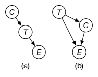
In Figure 11.9(a), $C$ is used to select which treatment was chosen (e.g., $C$ might be the student’s prior knowledge). In this case, the data for each condition is appropriate, so based on the data of Example 11.9, it is better to use the method.

In Figure 11.9(b), $C$ is a consequence of the treatment, such as whether the students learned a particular technique. In this case, the aggregated data is appropriate, so based on the data of Example 11.9, it is better not to use the method.

The best treatment is not only a function of the data, but also of the assumed causality.

Artificial Intelligence 3E