11 Causality 11 Causality 11.2 Missing Data

11.1 Probabilistic Causal Models

A direct cause of variable $Y$ is a variable $X$ such that intervening on $X$ , holding all other variables constant, can affect $Y$ . For example, if making rain would affect whether there is mud, with all other variables fixed, then rain is a direct cause of mud. If making mud does not affect rain, then mud is not a direct cause of rain.

Assume that there are no causal cycles. Examples of apparent causal cycles, such as poverty causes sickness and sickness causes poverty, are handled by considering time – each variable is about an event at some time; sickness at one time causes poverty at a future time, and poverty at one time causes sickness at future times.

Suppose you knew the direct causes of a variable and have not made any observations. The only way to affect the variable is to intervene on that variable or affect one of its direct causes. A variable is not independent of the variables it eventually causes, but is independent of the other variables given its direct causes. This is exactly the independence assumption of a belief network when the causes of each variable are before it in the total ordering of variables; thus, a belief network is an appropriate representation for a causal model. All of the reasoning in a belief network followed from that independence, and so is applicable to causal models.

A structural causal model defines a causal mechanism for each modeled variable. A causal mechanism defines a conditional probability for a variable given its parents, where the probability of the variable when the parents are set to some values by intervention is the same as it is when the parents are observed to have those values. For example, $P(light\_on\mid switch\_up)$ is a causal mechanism if the probability that the light is on is the same when intervening to make the light switch up as it is when observing it is up. $P(switch\_up\mid light\_off)$ would not be a causal mechanism if observing the light off results in a different belief about the switch than intervening to make the light off. Any of the representations for conditional probability can be used to represent causal mechanisms. A structural causal model defines a causal network, a belief network where the probability of each variable given its parents is the same when the parents are observed as when they are intervened on.

The following example is based on Pearl [2009, p. 15]:

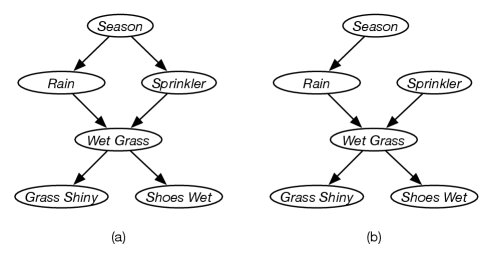
Refer to caption — Figure 11.1: Causal network causes of wet grass (a) and intervening by turning on the sprinkler (b)

Example 11.1.

Suppose some grass can be wet because of rain or a sprinkler. Whether it rains depends on the season. Whether the sprinkler was on also depends on the season. Wet grass causes it to be shiny and causes my shoes to get wet. A belief network for this story is given in Figure 11.1(a). Observing the sprinkler is on (or off) tells us something about the season (e.g., the sprinkler is more likely to be on during the dry season than the wet season), which in turn affects our belief in rain.

However, turning the sprinkler on or off does not affect (our belief in) the season. To model this intervention, replace the mechanism for the sprinkler, namely $P({Sprinkler}\mid{Season})$ , with $P({Sprinkler})$ , a deterministic conditional probability distribution (with probability 1 that the sprinkler is in the position selected), resulting in the network of Figure 11.1(b). This has the same probabilities for the season and rain as in (a) with no observations, but different probabilities for the remaining variables, as the probability the sprinkler is on has changed.

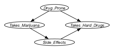
Example 11.2.

As discussed at the start of this chapter, taking marijuana and taking hard drugs are positively correlated. One possible causal relationship is given in Figure 11.2. A parametrization for this that fits the story below is given at AIPython (aipython.org). The side-effects may be ill effects or satisfying curiosity, both of which (for the point of this example) may decrease the appetite for hard drugs. Observing taking marijuana increases the probability of being drug prone and having side-effects, which in turn can increase the probability that the person takes hard drugs. This means that taking marijuana and taking hard drugs would be positively correlated. However, intervening to give someone marijuana would only increase the probability of side-effects (providing no information about whether they are drug prone), which in turn may decrease the probability that they take hard drugs. Similarly, depriving someone of marijuana (which would be an intervention making taking marijuana false) would increase the probability that they take hard drugs. You could debate whether this is a reasonable model, but with only observational data about the correlation between taking marijuana and taking hard drugs, it is impossible to infer the effect of intervening on taking marijuana.

11.1.1 Do-notation

The do-notation adds interventions to the language of probability:

P(x\mid do(z),y)

where $x$ , $y$ , and $z$ are propositions (possibly using complex formulas including conjunction) is the probability that $x$ is true after doing $z$ and then observing $y$ . (Intervening after observing is counterfactual reasoning because the intervention could make the observation no longer true.)

Example 11.3.

Consider Example 11.1, with the belief network of Figure 11.1(a). The probability that the shoes are wet given the sprinkler is (observed to be) on is

P(shoes\_wet\mid sprinkler)

which can be answered with standard probabilistic inference, as covered in Chapter 9. Observing the sprinkler is on can provide information about the season; $S p r i n k l e r$ and $S e a s o n$ have an arc between them in Figure 11.1(a).

The probability that shoes are wet given you turned the sprinkler on

P(shoes\_wet\mid do(sprinkler))

can be answered using probabilistic inference in the network of Figure 11.1(b) conditioned on $Sprinkler{\,{=}\,}true$ . Intervening on $S p r i n k l e r$ has no effect on $S e a s o n$ , because they are independent in this network.

The probability that the shoes are wet given that you turned the sprinkler on and then observed the grass was not shiny is given by

P(shoes\_wet\mid do(sprinkler),~{}\neg grass\_shiny)

which can be answered by conditioning on $s p r i n k l e r$ and $\neg grass\_shiny$ , and querying $Shoes\_wet$ in the graph of Figure 11.1(b).

The use of the do-notation allows you to ask questions about the manipulated graphs in terms of the original graph.

11.1.2 D-separation

The definition of a belief network – each variable is independent of the variables that are not its descendants given its parents – implies independencies among the variables. The graphical criterion used to determine independence is called d-separation.

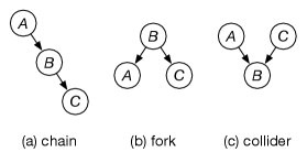
In a belief network, there are three ways two arcs can meet at a node, as shown in Figure 11.3, where an arc involving $A$ and $B$ meets an arc involving $B$ and $C$ .

Assuming that all arrows represent true dependency (the conditional probabilities do not imply more independencies than the graph):

(a)

In a chain ( $A\rightarrow B\rightarrow C$ ), $A$ and $C$ are dependent if $B$ is not observed, and are independent given $B$ . This is the same independence as the chain in the opposite direction ( $A\leftarrow B\leftarrow C$ ).
(b)

In a fork ( $A\leftarrow B\rightarrow C$ ), $A$ and $C$ are dependent if $B$ is not observed, and are independent given $B$ . This is the same independence structure as the chain; the chain and fork cannot be distinguished by observational data.
(c)

In a collider ( $A\rightarrow B\leftarrow C$ ), $A$ and $C$ are dependent given $B$ or one of its descendants. $A$ and $C$ are independent if $B$ and none of its descendants are observed.

Consider a path $p$ between two nodes in a directed acyclic graph, where the path can follow arcs in either direction. Recall that a path is a sequence of nodes where adjacent nodes in the sequence are connected by an arc. A set of nodes $Z$ blocks path $p$ if and only if

•

$p$ contains a chain ( $A\rightarrow B\rightarrow C$ or $A\leftarrow B\leftarrow C$ ) or a fork ( $A\leftarrow B\rightarrow C$ ) such that $B$ is in $Z$ , or
•

$p$ contains a collider ( $A\rightarrow B\leftarrow C$ ) such that $B$ is not in $Z$ and no descendant of $B$ is in $Z$ .

Nodes $X$ and $Y$ are d-separated by nodes $Z$ if $Z$ blocks every path from $X$ to $Y$ .

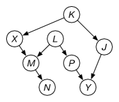
Example 11.4.

Consider the belief network of Figure 11.4. There are two paths between $X$ and $Y$ , both of which must be blocked for $X$ and $Y$ to be d-separated.

•

$X$ and $Y$ are not d-separated by $\{\}$ because the top path is not blocked.
•

$X$ and $Y$ are d-separated by $\{K\}$ because both paths are blocked
•

$X$ and $Y$ are not d-separated by $\{K,N\}$ because the bottom path is not blocked because $N$ is observed.
•

$X$ and $Y$ are d-separated by $\{K,N,P\}$ because both paths are blocked.

These independencies can be determined just from the graphical structure without considering the conditional distributions.

It can be proved that in a belief network, $X$ and $Y$ are independent given $Z$ for all conditional probability distributions if and only if $X$ and $Y$ are d-separated by $Z$ .

There can be independencies that hold even when d-separation doesn’t hold, due to the actual numbers in the conditional distributions. However, these are unstable in that changing the distribution slightly makes the variables dependent.

Artificial Intelligence 3E