Artificial
Intelligence 2E
foundations of computational agents
The third edition of Artificial Intelligence: foundations of computational agents, Cambridge University Press, 2023 is now available (including full text).
15.2.2 Learning Hidden Properties: Collaborative Filtering
Consider the problem of, given some tuples of a relation, predicting whether other tuples are true. Here we provide an algorithm that does this, even if there are no other relations defined.
In a recommender system users are given personalized recommendations of items they may like, and may not be aware of. One technique for recommender systems is predict the rating of a user on an item from the ratings of similar users or similar items, by what is called collaborative filtering.
One of the tasks for recommender systems is the top-n task, where is a positive integer, say 10, which is to present the user items they have not rated, and to judge the recommendation by how much the user likes one of these items. One way to select the items is to estimate the rating of each item for a user and to present the items with the highest predicted rating. An alternative is to take the diversity of the recommendations into account; it may be better to recommend very different items than to recommend similar items.
Example 15.15.
MovieLens (https://movielens.org/) is a movie recommendation system that acquires movie ratings from users. The rating is from 1 to 5 stars, where 5 stars is better. A data set for such a problem is of the form of Figure 15.3,
where each user is given a unique number, each item (movie) is given a unique number, and the timestamp is the Unix standard of seconds since 1970-01-01 UTC. These data can be used in a recommendation system to make predictions of other movies a user might like.
Consider the problem of predicting the rating for an item by a user. This prediction can be used to give personalized recommendations: recommend the items with the highest predicted ratings for a user on items they have not rated. The recommendations for each user may be different when they have provided different ratings. In the example above, the items were movies, but they could also be consumer goods, restaurants, holidays, or other items.
Netflix Prize
There was a considerable amount of research on collaborative filtering with the Netflix Prize to award $1,000,000 to the team that could improve the prediction accuracy of Netflix’s proprietary system, measured in terms of sum-of-squares by 10%. Each rating gives a user, a movie, the rating from 1 to 5 stars, and a date and time the rating was made. The data set consisted of approximately 100 million ratings from 480,189 anonymized users on 17,770 movies that was collected over a 7 year period. The prize was won in 2009 by a team that averaged over a collection of hundreds of predictors, some of which were quite sophisticated. After 3 years of research the winning team beat out another team by just 20 minutes to win the prize. They both had solutions which had essentially the same error, which was just under the threshold to win. Interestingly, an average of the two solutions was better than either alone.
The algorithm presented here is the basic algorithm that gave the most improvement.
The Netflix data set is no longer available because of privacy concerns. Although users were only identified by a number, there was enough information, if combined with other information, to potentially identify some of the users.
We develop an algorithm that does not take properties of the items or the users into account. It simply suggests items based on what other people have liked. It could potentially do better if it takes properties of the items and the users into account.
Suppose is a data set of triples, where means user gave item a rating of . (We are ignoring the timestamp here.) Let be the predicted rating of user on item . The aim is to optimize the sum-of-squares error:
which penalizes large errors much more than small errors. As with most machine learning, we want to optimize for the test examples, not for the training examples.
Here we give a sequence of more sophisticated predictions:
- Make a single prediction
-
In the simplest case, we could predict the same rating for all users and items: , where is the mean rating. Recall that if we are predicting the same for every user, predicting the mean minimizes the sum-of-squares error.
- Add user and item biases
-
Some users might give, on average, higher ratings than other users, and some movies may have higher ratings than other movies. We can take this into account using
where item has an item-bias parameter and user has a user-bias parameter . The parameters and are chosen to minimize the sum-of-squares error. If there are users and items, there are parameters to tune (assuming is fixed). Finding the best parameters is an optimization problem that can be done with a method like gradient descent, as was used for the linear learner.
One might think that should be directly related to the average rating for item and should be directly related to the average rating for user . However, it is possible that even if all of the ratings for user were above the mean . This can occur if user only rated very popular movies and rated them lower than other people.
Optimizing the and parameters can help get better estimates of the ratings, but it does not help in personalizing the recommendations, because the movies are still ordered the same for every user.
- Add a hidden property
-
We could hypothesize that there is an underlying property of users and movies that makes more accurate predictions. For example, we could have the age of users, and the age-appropriateness of movies. Instead of using observed properties, we can invent a hidden property and tune it to fit the data.
The hidden property has a value for item and a value for user . The product of these is used to predict the rating of that item for that user:
If and are both positive or both negative, the property will increase the prediction. If one or is negative and the other is positive, the property will decrease the prediction.
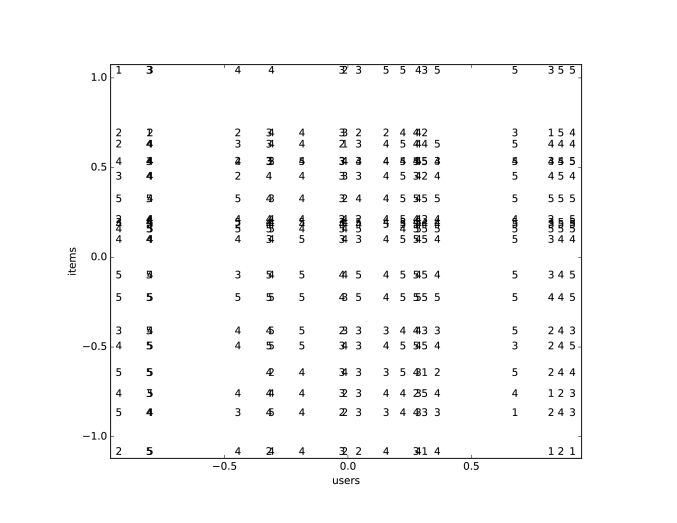
Figure 15.4: Movie ratings by users as a function of a single property Example 15.16.
Figure 15.4 shows a plot of the ratings as a function of a single property. This was for a subset of the MovieLens data set, where we selected 20 movies that had the most ratings, then we selected 20 users who had the most ratings for these movies. It was then trained for 1000 iterations of gradient descent, with a single property.
On the -axis are the users, ordered by their value, , on the property. On the -axis are the movies, ordered by their value, on the property. Each rating is then plotted against the user and the movie, so that triple is depicted by plotting at the position . Thus each vertical column of numbers corresponds to a user, and each horizontal row of numbers is a movie. The columns overlap if two users have very similar values on the property. The rows overlap for movies that have very similar values on the property. The users and the movies where the property values are close to zero are not affected by this property, as the prediction uses the product of values of the properties.
What we would expect is that generally high ratings are in the top-right and the bottom-left, as these are the ratings that are positive in the product, and low ratings in the top-left and bottom-right, as their product is negative. Note that what is high and low is relative to the user and movie biases; what is high for one movie may be different from what is high for another movie.
- Add hidden properties
-
There might not be just one property that makes users like movies, but there may be many such properties. Here we introduce such properties. There is a value for every item and property , and a value for every user and property . The contributions of the properties are added. This gives the prediction:
This is often called a matrix factorization method as the summation corresponds to matrix multiplication.
- Regularize
-
To avoid overfitting, a regularization term can be added to prevent the parameters from growing too much and overfitting the given data. Here an regularizer for each of the parameters is added to the optimization. The goal is to choose the parameters to
(15.1) where is a regularization parameter, which can be tuned by cross validation.
We can optimize the , , , and parameters using stochastic gradient descent. The algorithm is shown in Figure 15.5. Note that , need to be initialized randomly (and not to the same value) to force each property to be different.
This algorithm can be evaluated by how well it predicts future ratings. We can train it with the data up to a certain time, and test it on future data.
The algorithm can be improved in various ways including
-
•
taking into account observed attributes of items and users. This is important for the cold-start problem, which is how to make recommendations about new items or for new users
-
•
taking the timestamp into account, as users’ preferences may change and items may come in and out of fashion.