4.9.2 Local Search for Optimization

Local search is directly applicable to optimization problems, where the local search is used to minimize the objective function, rather than find a solution. The algorithm runs for a certain amount of time (perhaps including random restarts to explore other parts of the search space), always keeping the best assignment found thus far, and returning this as its answer.

Local search for optimization has one extra complication that does not arise when there are only hard constraints. With only hard constraints, the algorithm has found a solution when there are no conflicts. For optimization, is difficult to determine whether the best total assignment found is the best possible solution. A local optimum is a total assignment that is at least as good, according to the optimality criterion, as any of its possible successors. A global optimum is a total assignment that is at least as good as all of the other total assignments. Without systematically searching the other assignments, the algorithm may not know whether the best assignment found so far is a global optimum or whether a better solution exists in a different part of the search space.

When using local search to solve constrained optimization problems, with both hard and soft constraints, it is often useful to allow the algorithm to violate hard constraints on the way to a solution. This is done by making the cost of violating a hard constraint some large, but finite value.

Continuous Domains

For optimization with continuous domains, a local search becomes more complicated because it is not obvious what the possible successor of a total assignment are.

For optimization where the evaluation function is continuous and differentiable, gradient descent can be used to find a minimum value, and gradient ascent can be used to find a maximum value. Gradient descent is like walking downhill and always taking a step in the direction that goes down the most; this is the direction a rock will tumble if let loose. The general idea is that the successor of a total assignment is a step downhill in proportion to the slope of the evaluation function $h$ . Thus, gradient descent takes steps in each direction proportional to the negative of the partial derivative in that direction.

In one dimension, if $X$ is a real-valued variable with the current value of $v$ , the next value should be

v-\eta*\left(\frac{dh}{dX}\right)(v),

•

$\eta$ , the step size, is the constant of proportionality that determines how fast gradient descent approaches the minimum. If $\eta$ is too large, the algorithm can overshoot the minimum; if $\eta$ is too small, progress becomes very slow.
•

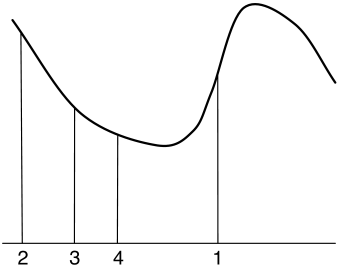
$\frac{dh}{dX}$ , the derivative of $h$ with respect to $X$ , is a function of $X$ and is evaluated for $X{=}v$ . This is equal to $\lim_{\epsilon\rightarrow 0}(h(X=v+\epsilon)-h(X=v))/\epsilon$

Example 4.31.

Figure 4.13 shows a typical example for finding a local minimum of a one-dimensional function. It starts at a position marked as 1. The derivative is a big positive value, so it takes a step to the left to position 2. Here the derivative is negative, and closer to zero, so it takes a smaller step to the right to position 3. At position 3, the derivative is negative and closer to zero, so it takes a smaller step to the right. As it approaches the local minimum value, the slope becomes closer to zero and it takes smaller steps.

For multidimensional optimization, when there are many variables, gradient descent takes a step in each dimension proportional to the partial derivative of that dimension. If $\left<X_{1},\ldots,X_{n}\right>$ are the variables that have to be assigned values, a total assignment corresponds to a tuple of values $\left<v_{1},\ldots,v_{n}\right>$ . The successor of the total assignment $\left<v_{1},\ldots,v_{n}\right>$ is obtained by moving in each direction in proportion to the slope of $h$ in that direction. The new value for $X_{i}$ is

v_{i}-\eta*\left(\frac{\partial h}{\partial X_{i}}\right)(v_{1},\ldots,v_{n}),

where $\eta$ is the step size. The partial derivative, $\frac{\partial h}{\partial X_{i}}$ , is a function of $X_{1},\dots,X_{n}$ . Applying it to the point $(v_{1},\ldots,v_{n})$ gives

\left(\frac{\partial h}{\partial X_{i}}\right)(v_{1},\ldots,v_{n})=\lim_{% \epsilon\rightarrow 0}\frac{h(v_{1},\dots,v_{i}+\epsilon,\dots,v_{n})-h(v_{1},% \dots,v_{i},\dots,v_{n})}{\epsilon}.

If the partial derivative of $h$ can be computed analytically, it is usually good to do so. If not, it can be estimated using a small value of $\epsilon$ .

Gradient descent is used for parameter learning, in which there may be thousands or even millions of real-valued parameters to be optimized. There are many variants of this algorithm. For example, instead of using a constant step size, the algorithm could do a binary search to determine a locally optimal step size.

For smooth functions, where there is a minimum, if the step size is small enough, gradient descent will converge to a local minimum. If the step size is too big, it is possible that the algorithm will diverge. If the step size is too small the algorithm will be very slow. If there is a unique local minimum, gradient descent, with a small enough step size, will converge to that global minimum. When there are multiple local minima, not all of which are global minima, it may need to search to find a global minimum, for example by doing a random restart or a random walk. These are not guarantee to find a global minimum unless the whole search space is exhausted, but are often as good as we can get.

Artificial Intelligence 2E

4.9.2 Local Search for Optimization

Continuous Domains

Example 4.31.

Artificial
Intelligence 2E