Artificial
Intelligence 2E
foundations of computational agents
The third edition of Artificial Intelligence: foundations of computational agents, Cambridge University Press, 2023 is now available (including full text).
7.3.2 Linear Regression and Classification
Linear functions provide a basis for many learning algorithms. This section first covers regression – the problem of predicting a real-valued function from training examples – then considers the discrete case of classification.
Linear regression is the problem of fitting a linear function to a set of training examples, in which the input and target features are numeric.
Suppose the input features, , are all numeric and there is a single target feature . A linear function of the input features is a function of the form
where is a tuple of weights. To make not be a special case, we invent a new feature, , whose value is always 1.
Suppose is a set of examples. The sum-of-squares error on examples for target is
| (7.1) |
In this linear case, the weights that minimize the error can be computed analytically (see Exercise 10). A more general approach, which can be used for wider classes of functions, is to compute the weights iteratively.
Gradient descent is an iterative method to find the minimum of a function. Gradient descent for minimizing starts with an initial set of weights; in each step, it decreases each weight in proportion to its partial derivative:
where , the gradient descent step size, is called the learning rate. The learning rate, as well as the features and the data, is given as input to the learning algorithm. The partial derivative specifies how much a small change in the weight would change the error.
The sum-of-squares error for a linear function is convex and has a unique local minimum, which is the global minimum. As gradient descent with small enough step size will converge to a local minimum, this algorithm will converge to the global minimum.
Consider minimizing the sum-of-squares error. The partial derivative of the error in Equation 7.1 with respect to weight is
| (7.2) |
where .
Gradient descent will update the weights after sweeping through all examples. An alternative is to update each weight after each example. Each example can update each weight using:
| (7.3) |
where we have ignored the constant 2, because we assume it is absorbed into the learning rate .
Figure 7.8 gives an algorithm, , for learning the weights of a linear function that minimize the sum-of-squares error. This algorithm returns a function that makes predictions on examples. In the algorithm, is defined to be 1 for all .
Termination is usually after some number of steps, when the error is small or when the changes get small.
Updating the weights after each example does not strictly implement gradient descent because the weights are changing beween examples. To implement gradient descent, we should save up all of the changes and update the weights after all of the examples have been processed. The algorithm presented in Figure 7.8 is called incremental gradient descent because the weights change while it iterates through the examples. If the examples are selected at random, this is called stochastic gradient descent. These incremental methods have cheaper steps than gradient descent and so typically become more accurate more quickly when compared to saving all of the changes to the end of the examples. However, it is not guaranteed that they will converge as individual examples can move the weights away from the minimum.
Batched gradient descent updates the weights after a batch of examples. The algorithm computes the changes to the weights after every example, but only applies the changes after the batch. If a batch is all of the examples, it is equivalent to gradient descent. If a batch consists of just one example, it is equivalent to incremental gradient descent. It is typical to start with small batches to learn quickly and then increase the batch size so that it converges.
A similar algorithm can be used for other error functions that are (almost always) differentiable and where the derivative has some signal (is not 0). For the absolute error, which is not differentiable at zero, the derivative can be defined to be zero at that point because the error is already at a minimum and the weights do not have to change. See Exercise 9. It does not work for other errors such as the 0/1 error, where the derivative is either 0 (almost everywhere) or undefined.
Squashed Linear Functions
Consider binary classification, where the domain of the target variable is . Multiple binary target variables can be learned separately.
The use of a linear function does not work well for such classification tasks; a learner should never make a prediction of greater than 1 or less than 0. However, a linear function could make a prediction of, say, 3 for one example just to fit other examples better.
A squashed linear function is of the form
where , an activation function, is a function from the real line into some subset of the real line, such as .
A prediction based on a squashed linear function is a linear classifier.
A simple activation function is the step function, , defined by
A step function was the basis for the perceptron [Rosenblatt, 1958], which was one of the early methods developed for learning. It is difficult to adapt gradient descent to step functions because gradient descent takes derivatives and step functions are not differentiable.
If the activation is (almost everywhere) differentiable, gradient descent can be used to update the weights. The step size might need to converge to zero to guarantee convergence.
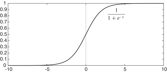
One differentiable activation function is the sigmoid or logistic function:
This function, depicted in Figure 7.9, squashes the real line into the interval , which is appropriate for classification because we would never want to make a prediction of greater than 1 or less than 0. It is also differentiable, with a simple derivative – namely, .
The problem of determining weights for the sigmoid of a linear function that minimize an error on a set of examples is called logistic regression.
To optimize the log loss error for logistic regression, minimize the negative log-likelihood
where .
where . This is, essentially, the same as Equation 7.2, the only differences being the definition of the predicted value and the constant “2” which can be absorbed into the step size.
The algorithm of Figure 7.8 can be modified to carry out logistic regression to minimize log loss by changing the prediction to be . The algorithm is show in Figure 7.10.
Example 7.11.
Consider learning a squashed linear function for classifying the data of Figure 7.1. One function that correctly classifies the examples is
where is the sigmoid function. A function similar to this can be found with about 3000 iterations of gradient descent with a learning rate . According to this function, is true (the predicted value for example is closer to 1 than 0) if and only if is true and either or is true. Thus, the linear classifier learns the same function as the decision tree learner. To see how this works, see the “mail reading” example of the Neural AIspace.org applet.
To minimize sum-of-squares error, instead, the prediction is the same, but the derivative is different. In particular, line 16 of Figure 7.10 should become
Consider each input feature as a dimension; if there are features, there will be dimensions. A hyperplane in an -dimensional space is a set of points that all satisfy a constraint that some linear function of the variables is zero. The hyperplane forms an -dimensional space. For example, in a (two-dimensional) plane, a hyperplane is a line, and in a three-dimensional space, a hyperplane is a plane. A classification is linearly separable if there exists a hyperplane where the classification is true on one side of the hyperplane and false on the other side.
The algorithm can learn any linearly separable classification. The error can be made arbitrarily small for arbitrary sets of examples if, and only if, the target classification is linearly separable. The hyperplane is the set of points where for the learned weights . On one side of this hyperplane, the prediction is greater than 0.5; on the other side, the prediction is less than 0.5.
Example 7.12.
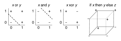
Figure 7.11 shows linear separators for “or” and “and”. The dashed line separates the positive (true) cases from the negative (false) cases. One simple function that is not linearly separable is the exclusive-or (xor) function. There is no straight line that separates the positive examples from the negative examples. As a result, a linear classifier cannot represent, and therefore cannot learn, the exclusive-or function.
Consider a learner with three input features , and , each with domain . Suppose that the ground truth is the function “if then else ”. This is depicted on the right of Figure 7.11 by a cube in the standard coordinates, where the , and range from 0 to 1. This function is not linearly separable.
Often it is difficult to determine a priori whether a data set is linearly separable.
Example 7.13.
Consider the data set of Figure 7.12 (a), which is used to predict whether a person likes a holiday as a function of whether there is culture, whether the person has to fly, whether the destination is hot, whether there is music, and whether there is nature. In this data set, the value 1 means true and 0 means false. The linear classifier requires the numerical representation.
| lin | |||||||
| 0 | 0 | 1 | 0 | 0 | 0 | 0.00011 | |
| 0 | 1 | 1 | 0 | 0 | 0 | 0.00011 | |
| 1 | 1 | 1 | 1 | 1 | 0 | 0.01121 | |
| 0 | 1 | 1 | 1 | 1 | 0 | 0.00113 | |
| 0 | 1 | 1 | 0 | 1 | 0 | 0.09279 | |
| 1 | 0 | 0 | 1 | 1 | 1 | 0.99015 | |
| 0 | 0 | 0 | 0 | 0 | 0 | 0.50250 | |
| 0 | 0 | 0 | 1 | 1 | 1 | 0.90970 | |
| 1 | 1 | 1 | 0 | 0 | 0 | 0.00113 | |
| 1 | 1 | 0 | 1 | 1 | 1 | 0.99024 | |
| 1 | 1 | 0 | 0 | 0 | 1 | 0.91052 | |
| 1 | 0 | 1 | 0 | 1 | 1 | 0.50250 | |
| 0 | 0 | 0 | 1 | 0 | 0 | 0.01110 | |
| 1 | 0 | 1 | 1 | 0 | 0 | 0.00001 | |
| 1 | 1 | 1 | 1 | 0 | 0 | 0.00001 | |
| 1 | 0 | 0 | 1 | 0 | 0 | 0.10065 | |
| 1 | 1 | 1 | 0 | 1 | 0 | 0.50500 | |
| 0 | 0 | 0 | 0 | 1 | 1 | 0.99890 | |
| 0 | 1 | 0 | 0 | 0 | 1 | 0.50500 | |
|
(a) |
(b) | ||||||
After 10,000 iterations of gradient descent with a learning rate of 0.05, the prediction found is (to one decimal point)
The linear function and the prediction for each example are shown in Figure 7.12 (b). All but four examples are predicted reasonably well, and for those four it predicts a value of approximately . This function is quite stable with different initializations. Increasing the number of iterations makes it predict the other tuples more accurately, but does not improve on these four. This data set is not linearly separable.
When the domain of the target variable has more than two values – there are more than two classes – indicator variables can be used to convert the classification to binary variables. These binary variables could be learned separately. The predictions of the individual classifiers can be combined to give a prediction for the target variable. Because exactly one of the values must be true for each example, a learner should not predict that more than one will be true or that none will be true. Suppose we separately learned the predicted values for are , where the . A learner that predicts a probability distribution could predict with probability . A learner that must make a definitive prediction can predict the mode, a for which is the maximum.