Artificial
Intelligence 2E
foundations of computational agents
The third edition of Artificial Intelligence: foundations of computational agents, Cambridge University Press, 2023 is now available (including full text).
7.4 Overfitting
Overfitting occurs when the learner makes predictions based on regularities that appear in the training examples but do not appear in the test examples or in the world from which the data is taken. It typically happens when the model tries to find signal in randomness – there are spurious correlations in the training data that are not reflected in the problem domain as a whole – or when the learner becomes overconfident in its model. This section outlines methods to detect and avoid overfitting.
Example 7.14.
Consider a website where people submit ratings for restaurants from 1 to 5 stars. Suppose the website designers would like to display the best restaurants, which are those restaurants that future patrons would like the most. It is extremely unlikely that a restaurant that has many ratings, no matter how outstanding it is, will have an average of 5 stars, because that would require all of the ratings to be 5 stars. However, given that 5 star ratings are not that uncommon, it would be quite likely that a restaurant with just one rating will have 5 stars. If the designers used the average rating, the top rated restaurants will be ones with very few ratings, and these are unlikely to be the best restaurants. Similarly, restaurants with few ratings but all low are unlikely to be as bad as the ratings indicate.
The phenomenon that extreme predictions will not perform as well on test cases is analogous to regression to the mean. Regression to the mean was discovered by Galton [1886], who called it regression to mediocrity, after discovering that the offspring of plants with larger than average seeds are more like average seeds than their parents are. In both of the restaurant and the seeds cases, this occurs because ratings, or the size, will be a mix of quality and luck (e.g., who gave the rating or what genes the seeds had). Restaurants that have a very high rating will have to be high in quality and be lucky (and be very lucky if the quality is not very high). More data averages out the luck; it is very unlikely that someones luck does not run out. Similarly, the seed offspring do not inherit the part of the size of the seed that was due to random fluctuations.
Overfitting is also caused by model complexity: a more complex model, with more parameters, can virtually always fit data better than a simple model.
Example 7.15.
A polynomial of degree is of the form:
The linear learner can be used unchanged to learn the weights of the polynomial that minimize the sum-of-squares error, simply by using as the input features to predict .
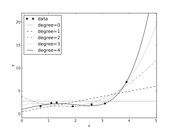
Figure 7.13 shows polynomials up to degree 4 for the data of Figure 7.2. Higher-order polynomials can fit the data better than lower-order polynomials, but that does not make them better on the training set.
Notice how the higher-order polynomials get more extreme in extrapolation. All of the polynomials, except the degree 0 polynomials, go to plus or minus infinity as gets bigger or smaller, which is almost never what you want. Moreover, if the maximum value of for which is even, then as approaches plus or minus infinity, the predictions will have the same sign, going to either plus infinity or minus infinity. The degree 4 polynomial in the figure approaches as gets smaller, which does not seems reasonable given the data. If the maximum value of for which is odd, then as approaches plus or minus infinity, the predictions will have opposite signs.
You need to be careful to use an appropriate step size to use gradient descent for such fitting polynomials. If is close to zero () then can be tiny, and if is is large () then can be enormous. Suppose in Figure 7.2 is in centimeters. If were in millimeters (so ), then the coefficient of would have a huge effect on the error. If were in meters (where ), the coefficient of would have very little effect on the error.
Example 7.14 showed how more data can allow for better predictions. Example 7.15 showed how complex models can lead to overfitting the data. We would like large amounts of data to make good predictions. However, even when we have so-called big data, the number of (potential) features tends to grow as well as the number of data points. For example, once there is a detailed enough description of patients, even if all of the people in the world were included, there would be no two patients that are identical in all respects.
The test set error is caused by:
-
•
bias, the error due to the algorithm finding an imperfect model. The bias is low when the model learned is close to the ground truth, the process in the world that generated the data. The bias can be divided into representation bias caused by the representation not containing a hypothesis close to the ground truth, and a search bias caused by the algorithm not searching enough of the space of hypotheses to find the appropriate hypothesis. For example, with discrete features, a decision tree can represent any function, and so has a low representation bias. With a large number of features, there are too many decision trees to search systematically, and decision tree learning can have a large search bias. Linear regression, if solved directly using the analytic solution, has a large representation bias, and zero search bias. There would also be a search bias if the gradient descent algorithm was used.
-
•
variance, the error due to a lack of data. A more complicated model, with more parameters to tune will require more data. Thus with a fixed amount of data, there is a bias–variance trade-off; we can have a complicated model which could be accurate, but we do not have enough data to estimate it appropriately (with low bias and high variance), or a simpler model that cannot be accurate, but we can estimate the parameters reasonably well given the data (with high bias and low variance).
-
•
noise the inherent error due to the data depending on features not modeled or because the process generating the data is inherently stochastic.
Overfitting results in overconfidence, where the learner is more confident in its prediction than the data warrants. For example, in the predictions in Figure 7.12, the probabilities are much more extreme than could be justified by the data. The first prediction, that there is approximately a 1 in 10000 chance of being true, does not seem to be reasonable given only 19 examples. This overconfidence is reflected in test data, as in the following example.
Example 7.16.
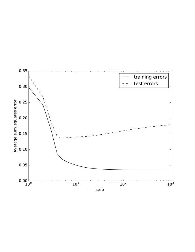
Figure 7.14 shows a typical plot of how the sum-of-squares error changes with the number of iterations of gradient descent. The sum-of-squares error on the training set decreases as the number of iterations increases. For the test set, the error reaches a minimum and then increases as the number of iterations increases. As it fits to the training examples, it becomes more confident in its imperfect model, and so errors in the test set become bigger.
The following sections discuss three ways to avoid overfitting. The first explicitly allows for regression to the mean, and can be used for cases where the representations are simple. The second provides an explicit trade-off between model complexity and fitting the data. The third approach is to use some of the training data to detect overfitting.