7.3 Basic Models for Supervised Learning 7.3 Basic Models for Supervised Learning 7.3.2 Linear Regression and Classification

The third edition of Artificial Intelligence: foundations of computational agents, Cambridge University Press, 2023 is now available (including full text).

7.3.1 Learning Decision Trees

A decision tree is a simple representation for classifying examples. Decision tree learning is one of the simplest useful techniques for supervised classification learning. For this section, assume there is a single discrete target feature called the classification. Each element of the domain of the classification is called a class.

A decision tree or a classification tree is a tree in which

•

each internal (non-leaf) node is labeled with a condition, a Boolean function of examples
•

each internal node has two children, one labeled with $t r u e$ and the other with $f a l s e$
•

each leaf of the tree is labeled with a point estimate on the class.

To classify an example, filter it down the tree, as follows. Each condition encountered in the tree is evaluated and the arc corresponding to the result is followed. When a leaf is reached, the classification corresponding to that leaf is returned. A decision tree corresponds to a nested if-then-else structure in a programming language.

Example 7.7.

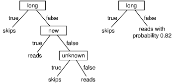
Figure 7.6 shows two possible decision trees for the examples of Figure 7.1. Each decision tree can be used to classify examples according to the user’s action. To classify a new example using the tree on the left, first determine the length. If it is long, predict $s k i p s$ . Otherwise, check the thread. If the thread is new, predict $r e a d s$ . Otherwise, check the author and predict $r e a d s$ only if the author is known. This decision tree can correctly classify all examples in Figure 7.1.

The tree corresponds to the program defining $\widehat{UserAction}({e})$ :

define $\widehat{UserAction}({e})$ :
	if $long(e)$ : return $s k i p s$
	else if $new(e)$ : return $r e a d s$
	else if $unknown(e)$ : return $s k i p s$
	else: return $r e a d s$

The tree on the right makes probabilistic predictions when the length is not $l o n g$ . In this case, it predicts $r e a d s$ with probability 0.82 and so $s k i p s$ with probability 0.18.

To use decision trees as a target representation, there are a number of questions that arise:

•

Given some training examples, what decision tree should be generated? Because a decision tree can represent any function of discrete input features, the bias that is necessary is incorporated into the preference of one decision tree over another. One proposal is to prefer the smallest tree that is consistent with the data, which could mean the tree with the least depth or the tree with the fewest nodes. Which decision trees are the best predictors of unseen data is an empirical question.
•

How should an agent go about building a decision tree? One way is to search the space of decision trees for the smallest decision tree that fits the data. Unfortunately, the space of decision trees is enormous (see Exercise 5). A practical solution is to carry out a greedy search on the space of decision trees, with the goal of minimizing the error. This is the idea behind the algorithm described below.

Searching for a Good Decision Tree

1: procedure Decision_tree_learner(

C s, Y, E s

)

2: Inputs

C s

: set of possible conditions

Y

: target feature

E s

: set of training examples

6: Output

7: function to predict a value of

Y

for an example

8: if stopping criterion is true then

9: let

v=point\_estimate(Y,Es)

10: define

T(e)=v

11: return

T

12: else

13: pick condition

c\in Cs

14:

true\_examples\;{:}{=}\;\mbox{}\{e\in Es:{c}({e})\}

15:

t_{1}\;{:}{=}\;\mbox{}Decision\_tree\_learner(Cs\setminus\{c\},Y,true\_examples)

16:

false\_examples\;{:}{=}\;\mbox{}\{e\in Es:\neg{c}({e})\}

17:

t_{0}\;{:}{=}\;\mbox{}Decision\_tree\_learner(Cs\setminus\{c\},Y,false\_examples)

18: define

T(e)=\mbox{ if }c(e)\mbox{ then }t_{1}(e)\mbox{ else }t_{0}(e)

19: return

T

Figure 7.7: Decision tree learner

The algorithm $Decision\_tree\_learner$ of Figure 7.7 builds a decision tree from the top down as follows. The input to the algorithm is a set of input conditions (Boolean functions of examples that use only input features), a target feature, and a set of training examples. If the input features are Boolean, they can be used directly as the conditions.

A decision tree can be seen as a simple branching program, taking in an example and returning a prediction for that example, either

•

a prediction that ignores the input conditions (a leaf) or
•

of the form “if $c(e)$ then $t_{1}(e)$ else $t_{0}(e)$ ” where $t_{1}$ and $t_{0}$ are decision trees; $t_{1}$ is the tree that is used when the condition $c$ is true of example $e$ , and $t_{0}$ is the tree used when $c(e)$ is false.

The learning algorithm mirrors this recursive decomposition of a tree. The learner first tests whether a stopping criterion is true. If the stopping criterion is true, it determines a point estimate for $Y$ , which is either a value for $Y$ or a probability distribution over the values for $Y$ . The function $point\_estimate(Y,Es)$ returns a value for $Y$ that can be predicted for all examples $E$ , ignoring the input features. The algorithm returns a function that returns that point estimate for any example. This is a leaf of the tree.

If the stopping criterion is not true, the learner picks a condition $c$ to split on, it partitions the training examples into those examples $e$ with $c(e)$ true and those examples with $\neg c(e)$ true (i.e., $c(e)=False$ ). It recursively builds a subtree for these sets of examples. It then returns a function that, given an example, tests whether $c$ is true of the example, and then uses the prediction from the appropriate subtree.

Example 7.8.

Consider applying $Decision\_tree\_learner$ to the classification data of Figure 7.1. The initial call is

	$\displaystyle{decisionTreeLearner(\{Author,Thread,Length,Where\_read\},User\_% action,}$
	$\displaystyle\ \ \ \ {\{e_{1},e_{2},\ldots,e_{18}\}).}$

Suppose the stopping criterion is not true and the algorithm picks the condition $Length=long$ to split on. It then calls

	$\displaystyle{decisionTreeLearner(\{Where\_read,Thread,Author\},User\_action,}$
	$\displaystyle\ \ \ \ {\{e_{1},e_{3},e_{4},e_{6},e_{9},e_{10},e_{12}\}).}$

All of these examples agree on the user action; therefore, the algorithm returns the prediction $s k i p s$ . The second step of the recursive call is

	$\displaystyle{decisionTreeLearner(\{Where\_read,Thread,Author\},User\_action,}$
	$\displaystyle\ \ \ \ {\{e_{2},e_{5},e_{7},e_{8},e_{11},e_{13},e_{14},e_{15},e_% {16},e_{17},e_{18}\}).}$

Not all of the examples agree on the user action, so assuming the stopping criterion is false, the algorithm picks a condition to split on. Suppose it picks $Thread=new$ . Eventually, this recursive call returns the function on example $e$ in the case when $L e n g t h$ is $s h o r t$ :

	$\displaystyle\mbox{if }new(e)$	$\displaystyle\mbox{ then }reads$
		$\displaystyle\mbox{ else if }unknown(e)\mbox{ then }skips\mbox{ else }reads$

The final result is the function of Example 7.7.

The learning algorithm of Figure 7.7 leaves three choices unspecified:

•
The stopping criterion is not defined. The learner needs to stop when there are no input conditions, or when all of the examples have the same classification. A number of criteria have been suggested for stopping earlier:
- –
  
  Minimum child size: do not split more if one of the children will have fewer examples than a threshold.
- –
  
  Minimum number of examples at a node: stop splitting if there are fewer examples than some threshold. With a minimum child size, we know we can stop with fewer than twice the minimum child size, but the threshold may be higher than this.
- –
  
  The improvement of the criteria being optimized must be above a threshold. For example, the information gain may need to be above some threshold.
- –
  
  Maximum depth: do not split more if the depth reaches a maximum.
•

What should be returned at the leaves is not defined. This is a point estimate that ignores all of the input conditions (except the ones on the path that lead to this leaf). This prediction is typically the most likely classification, the median value, the mean value, or a probability distribution over the classifications. See Exercise 8.
•

Which condition to pick to split on is not defined. The aim is to pick a condition that will result in the smallest tree. The standard way to do this is to pick the myopically optimal or greedy optimal split; if the learner were only allowed one split, pick whichever condition would result in the best classification if that were the only split. For likelihood, entropy, or when minimizing the log loss, the myopically optimal split is the one that gives the maximum information gain. Sometimes information gain is used even when the optimality criterion is some other error measure.

Example 7.9.

In the running example of learning the user action from the data of Figure 7.1, suppose you want to maximize the likelihood of the prediction or, equivalently, minimize the log loss. In this example, we myopically choose a split that minimizes the log loss.

Without any splits, the optimal prediction on the training set is the empirical frequency. There are $9$ examples with $User\_action{=}reads$ and $9$ examples with $User\_action{=}skips$ , and so $k n o w n$ is predicted with probability 0.5. The log loss is equal to $(-18*log_{2}0.5)/18=1$ .

Consider splitting on $A u t h o r$ . This partitions the examples into $[e_{1}$ , $e_{4}$ , $e_{5}$ , $e_{6}$ , $e_{9}$ , $e_{10}$ , $e_{12}$ , $e_{13}$ , $e_{14}$ , $e_{15}$ , $e_{16}$ , $e_{17}]$ with $Author{=}known$ and $[e_{2}$ , $e_{3}$ , $e_{7}$ , $e_{8}$ , $e_{11}$ , $e_{18}]$ with $Author{=}unknown$ , each of which is evenly split between the different user actions. The optimal prediction for each partition is again 0.5, and so the log loss after the split is again 1. In this case, finding out whether the author is known, by itself, provides no information about what the user action will be.

Splitting on $T h r e a d$ partitions the examples into $[e_{1}$ , $e_{2}$ , $e_{5}$ , $e_{8}$ , $e_{10}$ , $e_{12}$ , $e_{14}$ , $e_{15}$ , $e_{17}$ , $e_{18}]$ with $Thread{=}new$ and $[e_{3}$ , $e_{4}$ , $e_{6}$ , $e_{7}$ , $e_{9}$ , $e_{11}$ , $e_{13}$ , $e_{16}]$ with $Thread{=}followup$ . The examples with $Thread{=}new$ , contains $3$ examples with $User\_action{=}skips$ and $7$ examples with $User\_action{=}reads$ , thus the optimal prediction for these is to predict reads with probability $7/10$ . The examples with $Thread=followup$ , have 2 $r e a d s$ and 6 $s k i p s$ . Thus the best prediction for these is to predict $r e a d s$ with probability 2/8. The log loss after the split is

	$\displaystyle-(3\log_{2}(3/10)+7\log_{2}(7/10)+2\log_{2}(2/8)+6\log_{2}(6/% 8))/18$
	$\displaystyle\approx 15.3/18\approx 0.85$

Splitting on $L e n g t h$ divides the examples into $[e_{1}$ , $e_{3}$ , $e_{4}$ , $e_{6}$ , $e_{9}$ , $e_{10}$ , $e_{12}]$ and $[e_{2}$ , $e_{5}$ , $e_{7}$ , $e_{8}$ , $e_{11}$ , $e_{13}$ , $e_{14}$ , $e_{15}$ , $e_{16}$ , $e_{17}$ , $e_{18}]$ . The former all agree on the value of $User\_action$ and predict with probability 1. The user action divides the second set $9:2$ , and so the log loss is

-(7*\log_{2}1+9*\log_{2}9/11+2*\log_{2}2/11)/18\approx 7.5/18\approx 0.417

Therefore, splitting on $L e n g t h$ is better than splitting on $T h r e a d$ or $A u t h o r$ , when myopically optimizing the log loss.

In the algorithm of Figure 7.7, Boolean input features can be used directly as the conditions. Non-Boolean input features can be handled in two ways:

•

Expand the algorithm to allow multiway splits. To split on a multivalued variable, there would be a child for each value in the domain of the variable. This means that the representation of the decision tree becomes more complicated than the simple if-then-else form used for binary features. There are two main problems with this approach. The first is what to do with values of a feature for which there are no training examples. The second is that for most myopic splitting heuristics, including information gain, it is generally better to split on a variable with a larger domain because it produces more children and so can fit the data better than splitting on a feature with a smaller domain. However, splitting on a feature with a smaller domain keeps the representation more compact. A 4-way split, for example, is equivalent to 3 binary splits; they both result in 4 leaves. See Exercise 6.
•

Partition the domain of an input feature into two disjoint subsets, as with ordinal features or indicator variables

If the domain of input variable $X$ is totally ordered, a cut of the domain can be used as the condition. That is, the children could correspond to $X\leq v$ and $X>v$ for some value $v$ . To pick the optimal value for $v$ , sort the examples on the value of $X$ , and sweep through the examples to consider each split value and pick the best. See Exercise 7.

When the domain of $X$ is discrete and does not have a natural ordering, a split can be performed on arbitrary subsets of the domain. When the target is Boolean, each value of $X$ has a proportion of the target feature that is true. A myopically optimal split will be between values when the values are sorted according to this probability of the target feature.

A major problem of the preceding algorithm is overfitting the data. Overfitting occurs when the algorithm tries to fit distinctions that appear in the training data but do not appear in the test set. Overfitting is discussed more fully in Section 7.4.

There are two principal ways to overcome the problem of overfitting in decision trees:

•

Restrict the splitting to split only when the split is useful, such as only when the training-set error reduces by more than some threshold.
•

Allow unrestricted splitting and then prune the resulting tree where it makes unwarranted distinctions.

The second method often work better in practice. One reason is that it is possible that two features together predict well but one of them, by itself, is not very useful, as shown in the following example.

Example 7.10.

Matching pennies is a game where two coins are tossed and the player wins if both coins come up heads or both coins come up tails, and loses if the coins are different. Suppose the aim is to predict whether a game of matching pennies is won or not. The input features are $A$ , whether the first coin is heads or tails; $B$ , whether the second coin is heads or tails; and $C$ , whether there is cheering. The target feature, $W$ , is true when there is a win. Suppose cheering is correlated with winning. This example is tricky because $A$ by itself provides no information about $W$ , and $B$ by itself provides no information about $W$ . However, together they perfectly predict $W$ . A myopic split may first split on $C$ , because this provides the most myopic information. If all the agent is told is $C$ , this is much more useful than $A$ or $B$ . However, if the tree eventually splits on $A$ and $B$ , the split on $C$ is not needed. Pruning can remove $C$ as part of the tree, whereas stopping early will keep the split on $C$ .

A discussion of how to trade off model complexity and fit to the data is presented in Section 7.4.

Artificial Intelligence 2E