10.1.2 Probabilistic Classifiers

A Bayes classifier is a probabilistic model that is used for supervised learning. A Bayes classifier is based on the idea that the role of a class is to predict the values of features for members of that class. Examples are grouped in classes because they have common values for some of the features. Such classes are often called natural kinds. The learning agent learns how the features depend on the class and uses that model to predict the classification of a new example.

The simplest case is the naive Bayes classifier, which makes the independence assumption that the input features are conditionally independent of each other given the classification. The independence of the naive Bayes classifier is embodied in a belief network where the features are the nodes, the target feature (the classification) has no parents, and the target feature is the only parent of each input feature. This belief network requires the probability distributions $P(Y)$ for the target feature, or class, $Y$ and $P(X_{i}\mid Y)$ for each input feature $X_{i}$ . For each example, the prediction is computed by conditioning on observed values for the input features and querying the classification. Multiple target variables can be modeled and learned separately.

Figure 10.1: Belief network corresponding to a naive Bayes classifier

Example 10.3.

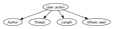
Suppose an agent wants to predict the user action given the data of Figure 7.1. For this example, the user action is the classification. The naive Bayes classifier for this example corresponds to the belief network of Figure 10.1. The input features form variables that are children of the classification.

Given an example with inputs $X_{1}{=}v_{1},\ldots,X_{k}{=}v_{k}$ , Bayes’ rule is used to compute the posterior probability distribution of the example’s classification, $Y$ :

	$\displaystyle P(Y\mid X_{1}$	$\displaystyle{=}v_{1},\ldots,X_{k}{=}v_{k})$
	$\displaystyle\mbox{}=\mbox{}$	$\displaystyle\frac{P(X_{1}{=}v_{1},\ldots,X_{k}{=}v_{k}\mid Y)*P(Y)}{P(X_{1}{=% }v_{1},\ldots,X_{k}{=}v_{k})}$
	$\displaystyle\mbox{}=\mbox{}$	$\displaystyle\frac{P(X_{1}{=}v_{1}\mid Y)\cdotsP(X_{k}{=}v_{k}\mid Y)P(Y)}{% \sum_{Y}P(X_{1}{=}v_{1}\mid Y)\cdotsP(X_{k}{=}v_{k}\mid Y)P(Y)}$
	$\displaystyle\mbox{}=\mbox{}$	$\displaystyle\frac{P(Y)\prod_{i=1}^{k}P(X_{i}{=}v_{i}\mid Y)P(Y)}{\sum_{Y}P(Y% )\prod_{i=1}^{k}P(X_{i}{=}v_{i}\mid Y)P(Y)}$

where the denominator is a normalizing constant to ensure the probabilities sum to 1.

Unlike many other models of supervised learning, the naive Bayes classifier can handle missing data where not all features are observed; the agent conditions on the features that are observed. Naive Bayes is optimal – it makes no independence assumptions – if only one of $X_{i}$ is observed, and as more of the $X_{i}$ are observed, the accuracy depends on how independent the $X_{i}$ are given $Y$ .

If every $X_{i}$ is observed, this model is the same as a logistic regression model, as the probability is proportional to a product, and so the logarithm is proportional to a sum. A naive Bayes model gives a direct way to assess the weights and allows for missing data. It however makes the assumption that the $X_{i}$ are independent given $Y$ , which may not hold. A linear regression model trained, for example, with gradient descent can take into account dependencies, but does not work for missing data.

Learning a Bayes Classifier

To learn a classifier, the distributions of $P(Y)$ and $P(X_{i}\mid Y)$ for each input feature can be learned from the data, as described in Section 10.1.1. Each conditional probability distribution $P(X_{i}\mid Y)$ may be treated as a separate learning problem for each value of $Y$ .

The simplest case is to use the maximum likelihood estimate (the empirical proportion in the training data as the probability), where $P(X_{i}{=}x_{i}\mid Y{=}y)$ is the number of cases where $X_{i}{=}x_{i}\wedge Y{=}y$ divided by the number of cases where $Y{=}y$ .

Example 10.4.

Suppose an agent wants to predict the user action given the data of Figure 7.1. For this example, the user action is the classification. The naive Bayes classifier for this example corresponds to the belief network of Figure 10.1. The training examples are used to determine the probabilities required for the belief network.

Suppose the agent uses the empirical frequencies as the probabilities for this example. The probabilities that can be derived from these data are

	$\displaystyle{P(User\_action{=}reads)=\ifrac{9}{18}=0.5}$
	$\displaystyle{P(Author{=}known\mid User\_action{=}reads)=\ifrac{2}{3}}$
	$\displaystyle{P(Author{=}known\mid User\_action{=}skips)=\ifrac{2}{3}}$
	$\displaystyle{P(Thread{=}new\mid User\_action{=}reads)=\ifrac{7}{9}}$
	$\displaystyle{P(Thread{=}new\mid User\_action{=}skips)=\ifrac{1}{3}}$
	$\displaystyle{P(Length{=}long\mid User\_action{=}reads)=0}$
	$\displaystyle{P(Length{=}long\mid User\_action{=}skips)=\ifrac{7}{9}}$
	$\displaystyle{P(Where\_read{=}home\mid User\_action{=}reads)=\ifrac{4}{9}}$
	$\displaystyle{P(Where\_read{=}home\mid User\_action{=}skips)=\ifrac{4}{9}~{}.}$

Based on these probabilities, the features $A u t h o r$ and $Where\_read$ have no predictive power because knowing either does not change the probability that the user will read the article. The rest of this example ignores these features.

To classify a new case where the author is unknown, the thread is a follow-up, the length is short, and it is read at home,

	$\displaystyle{P(User\_action{=}reads\mid Thread{=}followup\wedge Length{=}% short)}$
	$\displaystyle=P(followup\mid reads)P(short\mid reads)P(reads)*c$
	$\displaystyle=\ifrac{2}{9}1\ifrac{1}{2}*c$
	$\displaystyle=\ifrac{1}{9}*c$
	$\displaystyle{P(User\_action{=}skips\mid Thread{=}followup\wedge Length{=}% short)}$
	$\displaystyle=P(followup\mid skips)P(short\mid skips)P(skips)*c$
	$\displaystyle=\ifrac{2}{3}\ifrac{2}{9}\ifrac{1}{2}*c$
	$\displaystyle=\ifrac{2}{27}*c$

where $c$ is a normalizing constant. These must add up to 1, so $c$ is $\ifrac{27}{5}$ , thus

P(User\_action{=}reads\mid Thread{=}followup\wedge Length{=}short)=0.6~{}.

This prediction does not work well on example $e_{11}$ , which the agent skips, even though it is a $f o l l o w u p$ and is $s h o r t$ . The naive Bayes classifier summarizes the data into a few parameters. It predicts the article will be read because being short is a stronger indicator that the article will be read than being a follow-up is an indicator that the article will be skipped.

A new case where the length is long has a zero posterior probability that $User\_action{=}reads$ , no matter what the values of the other features. This is because $P(Length{=}long\mid User\_action{=}reads)=0$ .

The use of zero probabilities has some behaviors you may not want. First, some features become predictive: knowing just one feature value can rule out a category. A finite set of data might not be enough evidence to support such a conclusion. Second, if you use zero probabilities, it is possible that some combinations of observations are impossible, and the classifier will have a divide-by-zero error. See Exercise 1. This is a problem not necessarily with using a Bayes classifier but rather in using empirical frequencies as probabilities. The alternative to using the empirical frequencies is to incorporate pseudocounts. A designer of the learner should carefully choose pseudocounts, as shown in the following example.

Example 10.5.

Consider how to learn the probabilities for the help system of Example 8.35, where a helping agent infers what help page a user is interested in based on the words in the user’s query. The helping agent must learn the prior probability that each help page is wanted and the probability of each word given the help page wanted. These probabilities must be learned, because the system designer does not know a priori what words users will use in a query. The agent can learn from the words users actually use when looking for help. However, to be useful the system should also work before there are any data.

The learner must learn $P(H)$ . It could start with a pseudocount for each $h_{i}$ . Pages that are a priori more likely should have a higher pseudocount. If the designer did not have any prior belief about which pages were more likely, the agent could use the same pseudocount for each page. To think about what count to use, the designer should consider how much more the agent would believe a page is the correct page after it has seen the page once; see Section 7.4.1. It is possible to estimate this pseudocount if the designer has access to the data from another help system. Given the pseudocounts and some data, $P(h_{i})$ is computed by dividing the count (the empirical count plus the pseudocount) associated with $h_{i}$ by the sum of the counts for all the pages.

Similarly, the learner needs the probability $P(w_{j}\mid h_{i})$ , the probability that word $w_{j}$ will be used given the help page is $h_{i}$ . Because you may want the system to work even before it has received any data, the prior for these probabilities should be carefully designed, taking into account both the frequency of words in the language and the words in the help page itself.

Assume the following positive counts, which are observed counts plus suitable pseudocounts:

•

$c_{i}$ the number of times $h_{i}$ was the correct help page
•

$s=\sum_{i}c_{i}$ the total count
•

$u_{ij}$ the number of times $h_{i}$ was the correct help page and word $w_{j}$ was used in the query.

From these counts an agent can estimate the required probabilities:

	$\displaystyle P(h_{i})$	$\displaystyle=c_{i}/s$
	$\displaystyle P(w_{j}\mid h_{i})$	$\displaystyle=u_{ij}/c_{i}$

When a user claims to have found the appropriate help page, the counts for that page and the words in the query are updated. Thus, if the user indicates that $h_{i}$ is the correct page, the counts $s$ and $c_{i}$ are incremented, and for each word $w_{j}$ used in the query, $u_{ij}$ is incremented.

This model does not use information about the wrong page. If the user claims that a page is not the correct page, this information is not used.

Given a set of words, $Q$ , which the user issues as a query, the system can infer the probability of each help page:

	$\displaystyle P(h_{i}\mid Q)\propto\mbox{}$	$\displaystyle P(h_{i})\prod_{w_{j}\in Q}P(w_{j}\mid h_{i})\prod_{w_{j}\not% \in Q}(1-P(w_{j}\mid h_{i}))$
	$\displaystyle\mbox{}=\mbox{}$	$\displaystyle\frac{c_{i}}{s}\prod_{w_{j}\in Q}\frac{u_{ij}}{c_{i}}\prod_{w_{% j}\not\in Q}\frac{c_{i}-u_{ij}}{c_{i}}.$

The system could present the help page with the highest probability given the query. Note that it is important to use the words not in the query as well as the words in the query. For example, if a help page is about printing, the work “print” may be very likely to be used. The fact that “print” is not in a query is strong evidence that this is not the appropriate help page.

The calculation above is very expensive. It requires a product for all possible words, not just those words used in the query. This is problematic as there may be many possible words, and users want fast responses. It is possible to rewrite the above equation so that one product is over all the words, and to readjust for the words in the query:

	$\displaystyle P(h_{i}\mid Q)\propto\mbox{}$	$\displaystyle\frac{c_{i}}{s}\prod_{w_{j}\in Q}\frac{u_{ij}}{c_{i}}\prod_{w_{% j}\in Q}\frac{c_{i}}{c_{i}-u_{ij}}\prod_{w_{j}\in Q}\frac{c_{i}-u_{ij}}{c_{i}% }\prod_{w_{j}\not\in Q}\frac{c_{i}-u_{ij}}{c_{i}}$
	$\displaystyle\mbox{}=\mbox{}$	$\displaystyle\frac{c_{i}}{s}\prod_{w_{j}\in Q}\frac{u_{ij}}{c_{i}-u_{ij}}% \prod_{w_{j}}\frac{c_{i}-u_{ij}}{c_{i}}$
	$\displaystyle\mbox{}=\mbox{}$	$\displaystyle\Psi_{i}*\prod_{w_{j}\in Q}\frac{u_{ij}}{c_{i}-u_{ij}}$

where $\Psi_{i}=\frac{c_{i}}{s}*\prod_{w_{j}}\frac{c_{i}-u_{ij}}{c_{i}}$ does not depend on $Q$ and so can be computed offline. The fraction ${u_{ij}}/({c_{i}-u_{ij}})$ corresponds to the odds that word $w_{j}$ appears in page $h_{i}$ . The online calculation given a query only depends on the words in the query, which will be much faster than using all the words for reasonable queries.

The biggest challenge in building such a help system is not in the learning but in acquiring useful data. In particular, users may not know whether they have found the page they were looking for. Thus, users may not know when to stop and provide the feedback from which the system learns. Some users may never be satisfied with a page. Indeed, there may not exist a page they are satisfied with, but that information never gets fed back to the learner. Alternatively, some users may indicate they have found the page they were looking for, even though there may be another page that was more appropriate. In the latter case, the correct page may end up with its counts so low, it is never discovered. (See Exercise 2.)

Although there are some cases where the naive Bayes classifier does not produce good results, it is extremely simple, it is easy to implement, and often it works very well. It is a good method to try for a new problem.

In general, the naive Bayes classifier works well when the independence assumption is appropriate, that is, when the class is a good predictor of the other features and the other features are independent given the class. This may be appropriate for natural kinds, where the classes have evolved because they are useful in distinguishing the objects that humans want to distinguish. Natural kinds are often associated with nouns, such as the class of dogs or the class of chairs.

The naive Bayes classifier can be expanded to allow some input features to be parents of the classification and to allow some to be children. The probability of the classification given its parents could be represented as a decision tree or a squashed linear function or a neural network. The children of the classification do not have to be independent. One representation of the children is as a tree augmented naive Bayes (TAN) network, where the children are allowed to have exactly one other parent other than the classification (as long as the resulting graph is acyclic). This allows for a simple model that accounts for interdependencies among the children. An alternative is to put structure in the class variable. A latent tree model decomposes the class variable into a number of latent variables that are connected together in a tree structure. Each observed variable is a child of one of the latent variables. The latent variables allow a model of the dependence between the observed variables.

Artificial Intelligence 2E

10.1.2 Probabilistic Classifiers

Example 10.3.

Learning a Bayes Classifier

Example 10.4.

Example 10.5.

Artificial
Intelligence 2E