8.5 Sequential Probability Models 8.5.5 Time Granularity 8.6 Stochastic Simulation

The third edition of Artificial Intelligence: foundations of computational agents, Cambridge University Press, 2023 is now available (including full text).

8.5.6 Probabilistic Models of Language

Markov chains are the basis of simple language models, which have proved to be very useful in various natural language processing tasks in daily use.

Assume that a document is a sequence of sentences, where a sentence is a sequence of words. Here we want to consider the sorts of sentences that people may speak to a system or ask as a query to a help system. We do not assume they are grammatical, and often contain words, such as “thx” or “zzz”, which may not be typically thought of as words.

In the set-of-words model, a sentence (or a document) is treated as the set of words that appear in the sentence, ignoring the order of the words or whether the words are repeated. For example, the sentence “how can I phone my phone” would be treated as the set $\{$ “can”, “how”, “I”, “my”, “phone” $\}$ .

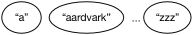
$domain("a")=domain("aardvark)=\dots=domain("zzz")=\{true,false\}$

Figure 8.19: Set-of-words language model

To represent the set-of-words model as a belief network, as in Figure 8.19, there is a Boolean random variable for each word. In this figure, the words are independent of each other (but they do not have to be). This belief network requires the probability of each word appearing in a sentence: $P("a")$ , $P("aardvark")$ , …, $P("zzz")$ . To condition on the sentence “how can I phone my phone”, all of the words in the sentence are assigned true, and all of the other words are assigned false. Words that are not defined in the model are either ignored, or are given a default (small) probability. The probability of sentence $S$ is $\left(\prod_{w\in S}P(w)\right)*\left(\prod_{w\not\in S}(1-P(w))\right)$ .

A set-of-words model is not very useful by itself, but is often used as part of a larger model, as in the following example.

Example 8.35.

Suppose we want to develop a help system to determine which help page users are interested in based on the keywords they give in a query to a help system.

The system will observe the words that the user gives. Instead of modeling the sentence structure, assume that the set of words used in a query will be sufficient to determine the help page.

The aim is to determine which help page the user wants. Suppose that the user is interested in one and only one help page. Thus, it seems reasonable to have a node $H$ with domain the set of all help pages, $\{h_{1},\dots,h_{k}\}$ .

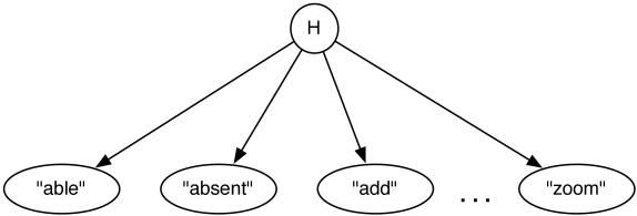
One way this could be represented is as a naive Bayes classifier. A naive Bayes classifier is a belief network that has a single node – the class – that directly influences the other variables, and the other variables are independent of each other given the class. Figure 8.20 shows a naive Bayes classifier for the help system where $H$ , the help page the user is interested in, is the class, and the other nodes represent the words used in the query. This network embodies the independence assumption: the words used in a query depend on the help page the user is interested in, and the words are conditionally independent of each other given the help page.

Figure 8.20: Naive belief network with a set-of-words model for a help system

This network requires $P(h_{i})$ for each help page $h_{i}$ , which specifies how likely it is that a user would want this help page given no information. This network assumes the user is interested in exactly one help page, and so $\sum_{i}P(h_{i})=1$ .

The network also requires, for each word $w_{j}$ and for each help page $h_{i}$ , the probability $P(w_{j}\mid h_{i})$ . These may seem more difficult to acquire but there are a few heuristics available. The sum of these values should be the average number of words in a query. We would expect words that appear in the help page to be more likely to be used when asking for that help page than words not in the help page. There may also be keywords associated with the page that may be more likely to be used. There may also be some words that are just used more, independently of the help page the user is interested in. Example 10.5 shows how to learn the probabilities of this network from experience.

To condition on the set of words in a query, the words that appear in the query are observed to be true and the words that are not in the query are observed to be false. For example, if the help text was “the zoom is absent”, the words “the”, “zoom”, “is”, and “absent” would be observed to be true, and the other words would be observed to be false. Once the posterior for $H$ has been computed, the most likely few help topics can be shown to the user.

Some words, such as “the” and “is”, may not be useful in that they have the same conditional probability for each help topic and so, perhaps, would be omitted from the model. Some words that may not be expected in a query could also be omitted from the model.

Note that the conditioning included the words that were not in the query. For example, if page $h_{73}$ was about printing problems, we may expect that people who wanted page $h_{73}$ would use the word “print”. The non-existence of the word “print” in a query is strong evidence that the user did not want page $h_{73}$ .

The independence of the words given the help page is a strong assumption. It probably does not apply to words like “not”, where which word “not” is associated with is very important. There may even be words that are complementary, in which case you would expect users to use one and not the other (e.g., “type” and “write”) and words you would expect to be used together (e.g., “go” and “to”); both of these cases violate the independence assumption. It is an empirical question as to how much violating the assumptions hurts the usefulness of the system.

$domain(W_{i})=\{"a","aarvark",\dots,"zzz","\bot","?"\}$

Figure 8.21: Bag-of-words or unigram language model

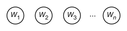
In a bag-of-words or unigram model, a sentence is treated as a multiset of words, representing the number of times a word is used in a sentence, but not the order of the words. Figure 8.21 shows how to represent a unigram as a belief network. For the sequence of words, there is a variable $W_{i}$ for each position $i$ , with domain of each variable the set of all words, such as $\{"a","aardvark",\dots,"zzz"\}$ . The domain is often augmented with a symbol, “ $\bot$ ”, representing the end of the sentence, and with a symbol “?” representing a word that is not in the model.

To condition on the sentence “how can I phone my phone”, the word $W_{1}$ is observed to be “how”, the variable $W_{2}$ is observed to be “can”, etc. Word $W_{7}$ is assigned $\bot$ . Both $W_{4}$ and $W_{6}$ are assigned the value “phone”. There are no variables $W_{8}$ onwards.

The unigram model assumes a stationary distribution, where the prior distribution of $W_{i}$ is the same for each $i$ . The value of $P(W_{i}=w)$ is the probability that a randomly chosen word is $w$ . More common words have a higher probability than less common words.

$domain(W_{i})=\{"a","aarvark",\dots,"zzz","\bot","?"\}$

Figure 8.22: Bigram language model

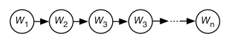
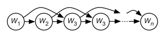
In a bigram model, the probability of each word depends on the previous word in the sentence. It is called a bigram model because it depends on pairs of words. Figure 8.22 shows the belief network representation of a bigram model. This needs a specification of $P(W_{i}\mid W_{i-1})$ .

To make $W_{1}$ not be a special case, we introduce a new word $\bot$ ; intuitively $\bot$ is the “word” between sentences. For example, $P("cat"\mid\bot)$ is the probability that the word “cat” is the first word in a sentence. $P(\bot\mid"cat")$ is the probability that the sentence ends after the the word “cat”.

In a trigram model, each triple of words is modeled. This is represented as a belief network in Figure 8.23. This requires $P(W_{i}\mid W_{i-2},W_{i-1})$ ; the probability of each word given the previous two words.

$W o r d$	$P_{1}$
the	0.0464
of	0.0294
and	0.0228
to	0.0197
in	0.0156
a	0.0152
is	0.00851
that	0.00806
for	0.00658
was	0.00508

$W o r d$	$P_{2}$
same	0.01023
first	0.00733
other	0.00594
most	0.00558
world	0.00428
time	0.00392
two	0.00273
whole	0.00197
people	0.00175
great	0.00102

$W o r d$	$P_{3}$
time	0.15236
as	0.04638
way	0.04258
thing	0.02057
year	0.00989
manner	0.00793
in	0.00739
day	0.00705
kind	0.00656
with	0.00327

Unigram, bigram and trigram probabilities derived from the Google books Ngram viewer (https://books.google.com/ngrams/) for the year 2000. $P_{1}$ is $P(Word)$ for the top 10 words, which are found by using the query “*” in the viewer. $P_{2}$ is part of a bigram model that represents $P(Word\mid"the")$ for the top 10 words. This is derived from the query “the *” in the viewer. $P_{3}$ is part of a trigram model; the probabilities given represent $P(Word\mid"the","same")$ , which is derived from the query “the same *” in the viewer.

Figure 8.24: Some of the most-likely n-grams

In general, in an n-gram model, the probability of each word given the previous $n-1$ words is modeled. This requires considering each sequence of $n$ words, and so the complexity of representing this as a table grows with $w^{n}$ where $w$ is the number of words. Figure 8.24 shows some common unigram, bigram and trigram probabilities.

The conditional probabilities are typically not represented as tables, because the tables would be too large, and because it is difficult to assess the probability of a previously unknown word, or the probability of the next word given a previously unknown word or given an uncommon phrase. Instead one could use context specific independence, such as, for trigram models, represent the probability of the next work conditioned on some of the pairs of words, and if none of these hold, use $P(W_{i}\mid W_{i-1})$ , as in a bigram model. For example, the phrase “frightfully green” is not common, and so to compute the probability of the next word, $P(W\mid"frightfully","green")$ , it is typical to use $P(W\mid"green")$ , which is easier to assess and learn.

Any of these models could be used in the help system of Example 8.35, instead of the set-of-words model used there. These models may be combined to give more sophisticated models, as in the following example.

Example 8.36.

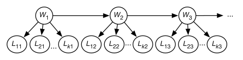
Consider the problem of spelling correction as users type into a phone’s onscreen keyboard to create sentences. Figure 8.25 gives a predictive typing model that does this (and more).

The variable $W_{i}$ is the $i$ th word in the sentence. The domain of each $W_{i}$ is the set of all words. This uses a bigram model for words, and assumes $P(W_{i}\mid W_{i-1})$ is provided as the language model. A stationary model is typically appropriate.

The $L_{ji}$ variable represents the $j$ th letter in word $i$ . The domain of each $L_{ji}$ is the set of characters that could be typed. This uses a unigram model for each letter given the word, but it would not be a stationary model, as for example, the probability distribution of the first letter given the word “print” is different from the probability distribution of the second letter given the word “print”. We would expect $P(L_{ji}=c\mid W_{i}=w)$ to be close to 1 if the $j$ th letter of word $w$ is $c$ . The conditional probability could incorporate common misspellings and common typing errors (e.g., switching letters, or if someone tends to type slightly higher on the phone’s screen).

For example, $P(L_{1j}="p"\mid W_{j}="print")$ would be close to 1, but not equal to 1, as the user could have mistyped. Similarly, $P(L_{2j}="r"\mid W_{j}="print")$ would be high. The distribution for the second letter in the word, $P(L_{2j}\mid W_{j}="print")$ , could take into account mistyping adjacent letters (“e” and “t” are adjacent to “r” on the standard keyboard), and missing letters (maybe “i” is more likely because it is the third letter in “print”). In practice, these probabilities are typically extracted from data of people typing known sentences, without needing to model why the errors occurred.

The word model allows the system to predict the next word even if no letters have been typed. Then as letters are typed, it predicts the word, based on the previous words and the typed letters, even if some of the letters are mistyped. For example, if the user types “I cannot pint”, it might be more likely that the last word is “print” than it is “pint” because of the way the model combines of all of the evidence.

A topic model predicts the topics of a document from the sentences typed. Knowing the topic of a document helps people find the document or similar documents even if they do not know what words are in the document.

Example 8.37.

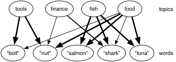
Figure 8.26 shows a simple topic model based on a set-of-words language model. There is a set of topics which are a priori independent of each other (four are given). The words are independent of each other given the topic. We assume a noisy-or model for how the words depend on the topics.

The noisy-or model can be represented by having a variable for each topic–word pair where the word is relevant for the topic. For example the $tools\_bolt$ variable represents the probability that the word $b o l t$ is in the document because the topic is $t o o l s$ . This variable has probability zero if the topic is not $t o o l s$ and has the probability that the word would appear when the topic is $t o o l s$ (and there are no other relevant topics). The word $b o l t$ would appear, with probability 1 if $tools\_bolt$ is true or if an analogous variable, $food\_bolt$ is true, and with a small probability otherwise (the probability that it appears without one of the topics). Thus, each topic–word pair where the word is relevant to the topic is modeled by a single weight. In Figure 8.26, the higher weights are show by thicker lines.

Given the words, the topic model is used to infer the distribution over topics. Once a number of words that are relevant a topic are given, the topic becomes more likely, and so other words related to that topic also become more likely. Indexing documents by the topic lets us find relevant documents even if different words are used to look for a document.

This model is based on Google’s Rephil, which has 12,000,000 words (where common phrases are treated as words), 900,000 topics and 350 million topic-word pairs with non-zero probability.

It is possible to mix these patterns, for example by using the current topics to predict the word in a predictive typing model with a topic model.

Models based on n-grams cannot represent all of the subtleties of natural language, as exemplified by the following example.

Example 8.38.

Consider the sentence:

A tall man with a big hairy cat drank the cold milk.

In English, this is unambiguous; the man drank the milk. Consider how an n-gram might fare with such a sentence. The problem is that the subject (“man”) is far away from the verb (“drank”). It is also plausible that the cat drank the milk. It is easy to think of variants of this sentence where the “man” is arbitrarily far away from the subject and so would not be captured by any n-gram. How to handle such sentences is discussed in Section 13.6.

Artificial Intelligence 2E

8.5.6 Probabilistic Models of Language

Example 8.35.

Example 8.36.

Example 8.37.

Example 8.38.

Artificial
Intelligence 2E