Artificial
Intelligence 2E
foundations of computational agents
The third edition of Artificial Intelligence: foundations of computational agents, Cambridge University Press, 2023 is now available (including full text).
8.4.2 Representing Conditional Probabilities and Factors
A conditional probability distribution is a function on variables; given an assignment to the values of the variables, it gives a number. A factor is a function of a set of variables; the variables it depends on are the scope of the factor. Thus a conditional probability is a factor, as it is a function on variables. This section explores some variants for representing factors and conditional probabilities. Some of the representations are for arbitrary factors and some are specific to conditional probabilities.
Factors do not have to be implemented as conditional probability tables. The resulting tabular representation is often too large when there are many parents. Often, structure in conditional probabilities can be exploited.
One such structure exploits context-specific independence, where one variable is conditionally independent of another, given a particular value of the third variable.
Example 8.25.
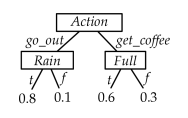
Suppose a robot can go outside or get coffee (so the has domain . Whether it gets wet (variable ) depends on whether there is rain (variable ) in the context that it went out or on whether the cup was full (variable ) if it got coffee. Thus is independent of given , but is dependent on given . Also, is independent of given , but is dependent on given .
Context-specific independence may be exploited in a representation by not requiring numbers that are not needed. A simple representation for conditional probabilities that models context-specific independence is a decision tree, where the parents in a belief network correspond to the input features and the child corresponds to the target feature. Another representation is in terms of definite clauses with probabilities. Context-specific independence could also be represented as tables that have contexts that specify when they should be used, as in the following example.
Example 8.26.
The conditional probability could be represented as a decision tree, as definite clauses with probabilities, or as tables with contexts:
Another common representation is a noisy-or, where the child is true if one of the parents is activated and each parent has a probability of activation. So the child is an “or” of the activations of the parents. The noisy-or is defined as follows. If has Boolean parents , the probability is defined by parameters . We invent new Boolean variables , where for each , has as its only parent. Define and . The bias term, has . The variables are the parents of , and the conditional probability is that is 1 if any of the are true and is 0 if all of the are false. Thus is the probability of when all of are false; the probability of increases if more of the become true.
Example 8.27.
Suppose the robot could get wet from rain or coffee. There is a probability that it gets wet from rain if it rains, and a probability that it gets wet from coffee if it has coffee, and a probability that it gets wet for other reasons. The robot gets wet if it gets wet from one of them, giving the “or”. We could have, , and, for the bias term, . The robot is wet if it wet from rain, wet from coffee, or wet for other reasons.
A log-linear model is a model where probabilities are specified as a product of terms. When the terms are non-zero (they are all strictly positive), the log of a product is the sum of logs. The sum of terms is often a convenient term to work with. To see how such a form is used to represent conditional probabilities, we can write the conditional probability in the following way:
-
•
The sigmoid function, , plotted in Figure 7.9, has been used previously in this book for logistic regression and neural networks.
-
•
The conditional odds (as often used by bookmakers in gambling) is
where is the prior odds and is the likelihood ratio. For a fixed , it is often useful to represent as a product of terms, and so the log is a sum of terms.
The logistic regression model of a conditional probability is of the form
where is assumed to have domain . (Assume a dummy input which is always 1.) This corresponds to a decomposition of the conditional probability, where the probabilities are a product of terms for each .
Note that . Thus determines the probability when all of the parents are zero. Each specifies a value that should be added as changes. If is Boolean with values , then . The logistic regression model makes the independence assumption that the influence of each parent on the child does not depend on the other parents. Learning logistic regression models was the topic of Section 7.3.2.
Example 8.28.
To represent the probability of given whether there is rain, coffee, kids, or whether the robot has a coat may be given by:
This implies the following conditional probabilities
This requires fewer parameters than the parameters required for a tabular representation, but makes more independence assumptions.
Noisy-or and logistic regression models are similar, but different. Noisy-or is typically used when the causal assumption that a variable is true if it is caused to be true by one of the parents, is appropriate. Logistic regression is used when the various parents add-up to influence the child.