Artificial
Intelligence 2E
foundations of computational agents
The third edition of Artificial Intelligence: foundations of computational agents, Cambridge University Press, 2023 is now available (including full text).
7.5 Neural Networks and Deep Learning
Neural networks are a popular target representation for learning. These networks are inspired by the neurons in the brain but do not actually simulate neurons. Artificial neural networks typically contain many fewer than the approximately neurons that are in the human brain, and the artificial neurons, called units, are much simpler than their biological counterparts. Neural networks have had considerable success in low-level reasoning for which there is abundant training data such as for image interpretation, speech recognition and machine translation. One reason is that they are very flexible and can invent features.
Artificial neural networks are interesting to study for a number of reasons:
-
•
As part of neuroscience, to understand real neural systems, researchers are simulating the neural systems of simple animals such as worms, which promises to lead to an understanding about which aspects of neural systems are necessary to explain the behavior of these animals.
-
•
Some researchers seek to automate not only the functionality of intelligence (which is what the field of artificial intelligence is about) but also the mechanism of the brain, suitably abstracted. One hypothesis is that the only way to build the functionality of the brain is by using the mechanism of the brain. This hypothesis can be tested by attempting to build intelligence using the mechanism of the brain, as well as attempting it without using the mechanism of the brain. Experience with building other machines, such as flying machines, which use the same principles, but not the same mechanism, that birds use to fly, would indicate that this hypothesis may not be true. However, it is interesting to test the hypothesis.
-
•
The brain inspires a new way to think about computation that contrasts with traditional computers. Unlike conventional computers, which have a few processors and a large but essentially inert memory, the brain consists of a huge number of asynchronous distributed processes, all running concurrently with no master controller. Conventional computers are not the only architecture available for computation. Indeed, current neural network systems are often implemented on massively parallel architectures.
-
•
As far as learning is concerned, neural networks provide a different measure of simplicity as a learning bias than, for example, decision trees. Multilayer neural networks, like decision trees, can represent any function of a set of discrete features. However, the functions that correspond to simple neural networks do not necessarily correspond to simple decision trees. Which is better, in practice, is an empirical question that can be tested on different problem domains.
There are many different types of neural networks. This book considers feed-forward neural networks. Feed-forward networks can be seen as a hierarchy consisting of linear functions interleaved with activation functions.
Neural networks can have multiple input features and multiple target features. These features are all real valued. Discrete features can be transformed into indicator variables or ordinal features. The inputs feed into layers of hidden units, which can be considered as features that are never directly observed, but are useful for prediction. Each of these units is a simple function of the units in a lower layer. These layers of hidden units feed ultimately into predictions of the target features.
A typical architecture is shown in Figure 7.16. There are layers of units (shown as circles). On the bottom layer are the input units for the input features. On the top is the output layer that makes predictions for the target variables.
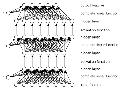
Each layer of units is a function of the previous layer. Each example has a value for each unit. We consider three kinds of layers:
-
•
An input layer consists of a unit for each input feature. This layer gets its value for an example from the value for the corresponding input feature for that example.
-
•
A complete linear layer, where each output is a linear function of the input values to the layer (and, as in linear regression, an extra constant input that has value “1” is added) defined by
for weights that are learned. There is a weight for every input–output pair of the layer. In the diagram of Figure 7.16 there is a weight for every arc for the linear functions.
-
•
An activation layer, where each output is a function of the corresponding input value, ; thus for activation function . Typical activation functions are the sigmoid: and the rectified linear unit (ReLU): . An activation function should be (almost everywhere) differentiable.
For regression, where the prediction can be any real number, it is typical for the last layer to be a complete linear layer, as this allows the full range of values. For binary classification, where the output values can be mapped to , it is typical for the output to be a sigmoid function of its inputs; one reason is that we never not want to predict a value greater than one or less than zero.
There is no point in having linear layers adjacent to each other because a linear function of a linear function is a linear function.
Back-propagation implements stochastic gradient descent for all weights. Recall that stochastic gradient descent involves updating each weight by , for each example .
There are two properties of differentiation used in back-propagation:
-
•
Linear rule: the derivative of a linear function, , is given by:
so the derivative is the number that is multiplied by in the linear function.
-
•
Chain rule: if is a function of and function , which does not depend on , is applied to , then
where is the derivative of .
Learning consists of two passes through the network for each example:
-
•
Prediction: given the values on the inputs for each layer, compute a value for the outputs of the layer.
-
•
Back-propagation: go backwards through the layers to update all of the weights of the network (the weights in the linear layers).
Treating each layer as a separate module, each layer has to implement the forward prediction and, in the back-propagation pass, update the weights in the layer and provide an error term for the lower levels. Back-propagation is an implementation of the chain rule that computes the derivative for all weights with one backward sweep through the network.
To make this more modular, an extra error layer, can sit above the network. For each example, this layer takes as inputs the prediction of the network on the target features for that example and the actual values of the target features for the example, and outputs an error that is fed into the final layer. Suppose the output of the final layer is an array of predictions, such that is a prediction of the th target feature, and the observed value for the current example in the training set is . The sum-of-squares error for a particular example is
Consider a generic weight somewhere in the network. Note that (potentially) depends on and does not
The error that is back-propagated for the sum-of-squares error is (where the 2 is absorbed into the step size). Back-propagation is used to update the value of each weight when it has computed this value for . Note that this is the negative of the derivative, so we can think of this as gradient ascent; the reason to do this is that it is easy to remember that a positive error means that the value needs to be increased, and a negative error means the value needs to be decreased. Minimizing another error function, such as the log loss, would result in different initial errors.
The input to each layer in the back-propagation phase is an error term for each of its output units. This is the product of the weights from the higher layers (the product of the terms in the chain rule) to compute derivative of the error. For a linear layer, each weight is updated by the value of the incoming error multiplied by the input value associated with that weight. Each layer must also pass the error signal to the lower level. The chain rule specifies that error passed back to the lower level is the error into the layer multiplied by the derivative of the function of the layer.
Each layer implements:
which returns the
output values for the input values
, where error is an array of a value for
each output unit,
updates the weights and returns an array of errors for the input units.
Figure 7.17 shows the algorithm for a neural network learner that carries out back-propagation for networks with multiple layers of units. The variable is a sequence of layers, where the lowest layer has the same number of inputs as there are input features. Each subsequent layer has the number of inputs that is equal to the number of outputs of the previous layer. The number of output units of the final layer is the same as the number of target features.
For the linear layers, the back-propagation algorithm is similar to the linear learner of Figure 7.8, but the algorithm also takes into account multiple linear layers and activation layers. Intuitively, for each example, back-propagation involves simulating the network on that example. At each stage contains the values of one layer to be input to the next layer. The derivative of the sum-of-squares errors for the outputs becomes the first value of error. This error is then passed back through the layers. This algorithm computes the derivative of each weight with one sweep back through the network.
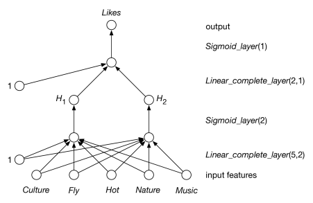
Example 7.20.
Consider training a network on the data of Figure 7.12. There are five input features and one output feature. Figure 7.18 shows a neural network represented by the following layers:
The lowest layer is a complete linear layer that takes five inputs and produces two outputs. The next sigmoid layer takes the sigmoid of these two outputs. Then a linear layer takes these and produces one linear output. The sigmoid of this output is the prediction of the network.
One run of back-propagation with the learning rate , and taking 10,000 steps, learns weights that accurately predict the training data. Each example gives (where weight are given to two significant digits):
Different runs can give quite different weights. For small examples like this, it is instructive to try to interpret the target; see Example 16.
The use of neural networks may seem to challenge the physical symbol system hypothesis, which relies on symbols having meaning. Part of the appeal of neural networks is that, although meaning is attached to the input and target units, the designer does not associate a meaning with the hidden units. What the hidden units actually represent is something that is learned. After a neural network has been trained, it is often possible to look inside the network to determine what a particular hidden unit actually represents. Sometimes it is easy to express concisely in language what it represents, but often it is not. However, arguably, the computer has an internal meaning; it can explain its internal meaning by showing how examples map into the values of the hidden unit, or by turning on one of the units in a layer and then simulating the rest of the network.
Using multiple layers in a neural network can be seen as a form of hierarchical modeling, in what has become known as deep learning. Convolutional neural networks are specialized for vision tasks, and recurrent neural networks are used for time series. A typical real-world network can have 10 to 20 layers with hundreds of millions of weights, which can take hours or days or months to learn on machines with thousands of cores.