Artificial
Intelligence 2E
foundations of computational agents
The third edition of Artificial Intelligence: foundations of computational agents, Cambridge University Press, 2023 is now available (including full text).
2.3 Hierarchical Control
One way that you could imagine building an agent depicted in Figure 2.1 is to split the body into the sensors and actuators, with a complex perception system that feeds a description of the world into a reasoning engine implementing a controller that, in turn, outputs commands to the actuators. This turns out to be a bad architecture for intelligent systems. It is too slow and it is difficult to reconcile the slow reasoning about complex, high-level goals with the fast reaction that an agent needs for lower-level tasks such as avoiding obstacles. It also is not clear that there is a description of a world that is independent of what you do with it (see Exercise 1).
 |
 |
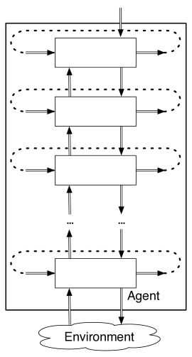
An alternative architecture is a hierarchy of controllers as depicted in Figure 2.4. Each layer sees the layers below it as a virtual body from which it gets percepts and to which it sends commands. The planning horizon at the lower level is much shorter than the planning horizon at upper levels. The lower-level layers run much faster, react to those aspects of the world that need to be reacted to quickly, and deliver a simpler view of the world to the higher layers, hiding details that are not essential for the higher layers. People have to react to the world, at the lowest level, in fractions of a second, but plan at the highest-level even for decades into the future. For example, the reason for doing some particular university course may be for the long-term career.
There is much evidence that people have multiple qualitatively different levels. Kahneman [2011] presents evidence for two distinct levels: System 1, the lower level, is fast, automatic, parallel, intuitive, instinctive, emotional, and not open to introspection, and System 2, the higher level, is slow, deliberate, serial, open to introspection, and based on reasoning.
In a hierarchical controller there can be multiple channels – each representing a feature – between layers and between layers at different times.
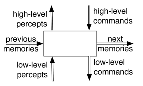
There are three types of inputs to each layer at each time:
-
•
the features that come from the belief state, which are referred to as the remembered or previous values of these features
-
•
the features representing the percepts from the layer below in the hierarchy
-
•
the features representing the commands from the layer above in the hierarchy.
There are three types of outputs from each layer at each time:
-
•
the higher-level percepts for the layer above
-
•
the lower-level commands for the layer below
-
•
the next values for the belief-state features.
An implementation of a layer specifies how the outputs of a layer are a function of its inputs. The definition of the belief state transition function and the command function can be extended to include higher-level commands as inputs, and each layer also requires a percept function, represented as tell below. Thus a layer implements:
where is the belief state, is the set of commands from the higher layer, is the set of percepts from the lower layer, is the set of commands for the lower layer, is the set of percepts for the higher layer.
Computing these functions can involve arbitrary computation, but the goal is to keep each layer as simple as possible.
To implement a controller, each input to a layer must get its value from somewhere. Each percept or command input should be connected to an output of some other layer. Other inputs come from the remembered beliefs. The outputs of a layer do not have to be connected to anything, or they could be connected to multiple inputs.
High-level reasoning, as carried out in the higher layers, is often discrete and qualitative, whereas low-level reasoning, as carried out in the lower layers, is often continuous and quantitative (see box). A controller that reasons in terms of both discrete and continuous values is called a hybrid system.
Qualitative Versus Quantitative Representations
Much of science and engineering considers quantitative reasoning with numerical quantities, using differential and integral calculus as the main tools. Qualitative reasoning is reasoning, often using logic, about qualitative distinctions rather than numerical values for given parameters.
Qualitative reasoning is important for a number of reasons.
-
•
An agent may not know what the exact values are. For example, for the delivery robot to pour coffee, it may not be able to compute the optimal angle that the coffee pot needs to be tilted, but a simple control rule may suffice to fill the cup to a suitable level.
-
•
The reasoning may be applicable regardless of the quantitative values. For example, you may want a strategy for a robot that works regardless of what loads are placed on the robot, how slippery the floors are, or what the actual charge is of the batteries, as long as they are within some normal operating ranges.
-
•
An agent needs to do qualitative reasoning to determine which quantitative laws are applicable. For example, if the delivery robot is filling a coffee cup, different quantitative formulas are appropriate to determine where the coffee goes when the coffee pot is not tilted enough for coffee to come out, when coffee comes out into a non-full cup, and when the coffee cup is full and the coffee is soaking into the carpet.
Qualitative reasoning uses discrete values, which can take a number of forms:
-
•
Landmarks are values that make qualitative distinctions in the individual being modeled. In the coffee example, some important qualitative distinctions include whether the coffee cup is empty, partially full, or full. These landmark values are all that is needed to predict what happens if the cup is tipped upside down or if coffee is poured into the cup.
-
•
Orders-of-magnitude reasoning involves approximate reasoning that ignores minor distinctions. For example, a partially full coffee cup may be full enough to deliver, half empty, or nearly empty. These fuzzy terms have ill-defined borders.
-
•
Qualitative derivatives indicate whether some value is increasing, decreasing, or staying the same.
A flexible agent needs to do qualitative reasoning before it does quantitative reasoning. Sometimes qualitative reasoning is all that is needed. Thus, an agent does not always need to do quantitative reasoning, but sometimes it needs to do both qualitative and quantitative reasoning.
Example 2.4.
Consider a delivery robot able to carry out high-level navigation tasks while avoiding obstacles. The delivery robot is required to visit a sequence of named locations in the environment of Figure 1.7, avoiding obstacles it may encounter.
Assume the delivery robot has wheels, like a car, and at each time can either go straight, turn right, or turn left. It cannot stop. The velocity is constant and the only command is to set the steering angle. Turning the wheels is instantaneous, but turning to a certain direction takes time. Thus, the robot can only travel straight ahead or go around in circular arcs with a fixed radius.
The robot has a position sensor that gives its current coordinates and orientation. It has a single whisker sensor that sticks out in front and slightly to the right and detects when it has hit an obstacle. In the example below, the whisker points to the right of the direction the robot is facing. The robot does not have a map, and the environment can change with obstacles moving.
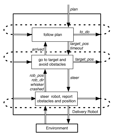
A layered controller for the delivery robot is shown in Figure 2.5. The robot is given a high-level plan to execute. The robot needs to sense the world and to move in the world in order to carry out the plan. The details of the lowest layer of the controller are not shown in this figure.
The top layer, called follow plan, is described in Example 2.6. That layer takes in a plan to execute. The plan is a list of named locations to visit in sequence. The locations are selected in order. Each selected location becomes the current target. This layer determines the - coordinates of the target. These coordinates are the target position for the middle layer. The top layer knows about the names of locations, but the lower layers only know about coordinates.
The top layer maintains a belief state consisting of a list of names of locations that the robot still needs to visit. It issues commands to the middle layer to go to the current target position but not to spend more than timeout steps. The percepts for the top layer are whether the robot has arrived at the target position or not. So the top layer abstracts the details of the robot and the environment.
The middle layer, which could be called go to target and avoid obstacles, tries to keep traveling toward the current target position, avoiding obstacles. The middle layer is described in Example 2.5. The target position, target_pos, is received from the top layer. The middle layer needs to remember the current target position it is heading towards. When the middle layer has arrived at the target position or has reached the timeout, it signals to the top layer whether the robot has arrived at the target. When arrived becomes true, the top layer can change the target position to the coordinates of the next location on the plan.
The middle layer can access the robot’s position, the robot’s direction and whether the robot’s whisker sensor is on or off. It can use a simple strategy of trying to head toward the target unless it is blocked, in which case it turns left.
The middle layer is built on a lower layer that provides a simple view of the robot. This lower layer could be called steer robot and report obstacles and position. It takes in steering commands and reports the robot’s position, orientation, and whether the whisker sensor is on or off.
Inside a layer are features that can be functions of other features and of the inputs to the layers. In the graphical representation of a controller, there is an arc into a feature from the features or inputs on which it is dependent. The features that make up the belief state can be written to and read from memory.
In the controller code in the following two examples, means that is the command for the lower level to do.
Example 2.5.
The middle go to location and avoid obstacles layer steers the robot towards a target position while avoiding obstacles. The inputs and outputs of this layer are given in Figure 2.6.
The layer receives two high-level commands: a target position to head towards and a timeout, which is the number of steps it should take before giving up. It signals the higher layer when it has arrived or when the timeout is reached.
The robot has a single whisker sensor that detects obstacles touching the whisker. The one bit value that specifies whether the whisker sensor has hit an obstacle is provided by the lower layer. The lower layer also provides the robot position and orientation. All the robot can do is steer left by a fixed angle, steer right, or go straight. The aim of this layer is to make the robot head toward its current target position, avoiding obstacles in the process, and to report when it has arrived.
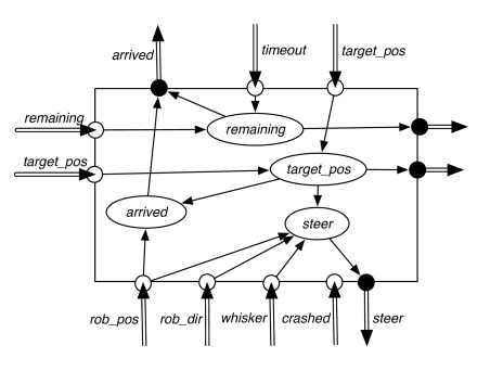
This layer of the controller needs to remember the target position and the number of steps remaining. The command function specifies the robot’s steering direction as a function of its inputs and whether the robot has arrived.
The robot has arrived if its current position is close to the target position. Thus, arrived is function of the robot position and previous target position, and a threshold constant:
where distance is the Euclidean distance, and threshold is a distance in the appropriate units.
The robot steers left if the whisker sensor is on; otherwise it heads toward the target position. This can be achieved by assigning the appropriate value to the variable, given an integer timeout and target_pos:
where is true when the robot is at rob_pos, facing the direction robot_dir, and when the current target position, target_pos, is straight ahead of the robot with some threshold (for later examples, this threshold is of straight ahead). The function left_of tests if the target is to the left of the robot.
Example 2.6.
The top layer, follow plan, is given a plan – a list of named locations to visit in order. These are the kinds of targets that could be produced by a planner, such as those that are developed in Chapter 6. The top layer must output target coordinates to the middle layer, and remember what it needs to carry out the plan. The layer is shown in Figure 2.7.
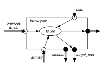
This layer remembers the locations it still has to visit. The to_do feature has as its value a list of all pending locations to visit.
Once the middle layer has signalled that the robot has arrived at its previous target or it has reached the timeout, the top layer gets the next target position from the head of the to_do list. The plan given is in terms of named locations, so these must be translated into coordinates for the middle layer to use. The following code shows the top layer as a function of the plan:
where is the first location in the to_do list, and is the rest of the to_do list. The function returns the coordinates of a named location loc. The controller tells the lower layer to go to the target coordinates, with a timeout here of 200 (which, of course, should be set appropriately). is true when the to_do list is empty.
This layer determines the coordinates of the named locations. This could be done by simply having a database that specifies the coordinates of the locations. Using such a database is sensible if the locations do not move and are known a priori. If the locations can move, the lower layer must be able to tell the upper layer the current position of a location. See Exercise 7.
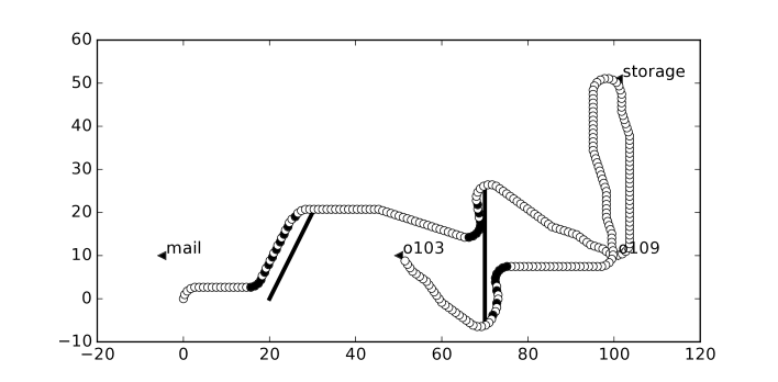
A simulation of the plan , , , with two obstacles is given in Figure 2.8. The robot starts at position facing North, and the obstacles are shown with lines. The agent does not know about the obstacles before it starts.
Each layer is simple, and none model the full complexity of the problem. But, together they exhibit complex behavior.