Third edition of Artificial Intelligence: foundations of computational agents, Cambridge University Press, 2023 is now available (including the full text).
11.1.3 EM for Soft Clustering
The EM algorithm can be used for soft clustering. Intuitively, for clustering, EM is like the k-means algorithm, but examples are probabilistically in classes, and probabilities define the distance metric. We assume here that the features are discrete.
As in the k-means algorithm, the training examples and the number of classes, k, are given as input.
When clustering, the role of the categorization is to be able to predict the values of the features. To use EM for soft clustering, we can use a naive Bayesian classifier, where the input features probabilistically depend on the class and are independent of each other given the class. The class variable has k values, which can be just {1,...,k}.
| Model | Data | → | Probabilities | |||||||||||||||||||||||||
 |
|
| ||||||||||||||||||||||||||
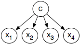
Given the naive Bayesian model and the data, the EM algorithm produces the probabilities needed for the classifier, as shown in Figure 11.2. The class variable is C in this figure. The probability distribution of the class and the probabilities of the features given the class are enough to classify any new example.
To initialize the EM algorithm, augment the data with a class feature, C, and a count column. Each original tuple gets mapped into k tuples, one for each class. The counts for these tuples are assigned randomly so that they sum to 1. For example, for four features and three classes, we could have the following:
| X1 | X2 | X3 | X4 |
| ... | ... | ... | ... |
| t | f | t | t |
| ... | ... | ... | ... |
-->
| X1 | X2 | X3 | X4 | C | Count |
| ... | ... | ... | ... | ... | ... |
| t | f | t | t | 1 | 0.4 |
| t | f | t | t | 2 | 0.1 |
| t | f | t | t | 3 | 0.5 |
| ... | ... | ... | ... | ... | ... |
If the set of training examples contains multiple tuples with the same values on the input features, these can be grouped together in the augmented data. If there are m tuples in the set of training examples with the same assignment of values to the input features, the sum of the counts in the augmented data with those feature values is equal to m.

The EM algorithm, illustrated in Figure 11.3, maintains both the probability tables and the augmented data. In the E step, it updates the counts, and in the M step it updates the probabilities.
2: Inputs
3: X set of features X={X1,...,Xn}
4: D data set on features {X1,...,Xn}
5: k number of classes Output
6: P(C), P(Xi|C) for each i∈{1:n}, where C={1,...,k}. Local
7: real array A[X1,...,Xn,C]
8: real array P[C]
9: real arrays Mi[Xi,C] for each i∈{1:n}
10: real arrays Pi[Xi,C] for each i∈{1:n}
11: s← number of tuples in D
12: Assign P[C], Pi[Xi,C] arbitrarily
13: repeat
14: // E Step
15: for each assignment ⟨X1=v1,...,Xn=vn⟩∈D do
16: let m ←|⟨X1=v1,...,Xn=vn⟩∈D|
17: for each c ∈{1:k} do
18: A[v1,...,vn,c]←m×P(C=c|X1=v1,...,Xn=vn)
19:
20:
21: // M Step
22: for each i∈{1:n} do
23: Mi[Xi,C]=∑X1,...,Xi-1,Xi+1,...,Xn A[X1,...,Xn,C]
24: Pi[Xi,C]=(Mi[Xi,C])/(∑C Mi[Xi,C])
25:
26: P[C]=∑X1,...,Xn A[X1,...,Xn,C]/s
27: until termination
The algorithm is presented in Figure 11.4. In this figure, A[X1,...,Xn,C] contains the augmented data; Mi[Xi,C] is the marginal probability, P(Xi,C), derived from A; and Pi[Xi,C] is the conditional probability P(Xi|C). It repeats two steps:
- E step: Update the augmented data based on the probability distribution. Suppose there are m copies
of the tuple
⟨X1=v1,...,Xn=vn⟩ in the
original data.
In the augmented data, the count associated with class c, stored in
A[v1,...,vn,c],
is updated to
m ×P(C=c|X1=v1,...,Xn=vn).
Note that this step involves probabilistic inference, as shown below.
- M step: Infer the maximum-likelihood probabilities for the model from the augmented data. This is the same problem as learning probabilities from data.
The EM algorithm presented starts with made-up probabilities. It could have started with made-up counts. EM will converge to a local maximum of the likelihood of the data. The algorithm can terminate when the changes are small enough.
This algorithm returns a probabilistic model, which can be used to classify an existing or new example. The way to classify a new example, and the way to evaluate line 18, is to use the following:
P(C=c|X1=v1,...,Xn=vn) = (P(C=c) ×∏i=1n P(Xi=vi|C=c))/(∑c'P(C=c') ×∏i=1n P(Xi=vi|C=c')) .
The probabilities in this equation are specified as part of the model learned.
Notice the similarity with the k-means algorithm. The E step (probabilistically) assigns examples to classes, and the M step determines what the classes predict.
In the M step, P(C=i) is set to the proportion of the counts with C=i, which is
(∑X1,...,Xn A[X1,...,Xn,C=i])/(m) ,
which can be computed with one pass through the data.
M1[X1,C], for example, becomes
∑X2,X3 ,X4 A[X1,...,X4,C].
It is possible to update all of the Mi[Xi,C] arrays with one pass though the data. See Exercise 11.3. The conditional probabilities represented by the Pi arrays can be computed from the Mi arrays by normalizing.
The E step updates the counts in the augmented data. It will replace the 0.4 in Figure 11.3 with
P(C=1|x1 ∧¬x2 ∧x3 ∧x4) = (P(x1|C=1) P(¬x2|C=1)P(x3|C=1)P(x4|C=1)P(C=1))/(∑i=13 P(x1|C=i) P(¬x2|C=i)P(x3|C=i)P(x4|C=i)P(C=i)) .
Each of these probabilities is provided as part of the learned model.
Note that, as long as k>1, EM virtually always has multiple local maxima. In particular, any permutation of the class labels of a local maximum will also be a local maximum.
