Third edition of Artificial Intelligence: foundations of computational agents, Cambridge University Press, 2023 is now available (including the full text).
11.1.2 k-Means
The k-means algorithm is used for hard clustering. The training examples and the number of classes, k, are given as input. The output is a set of k classes, a prediction of a value for each feature for each class, and an assignment of examples to classes.
The algorithm assumes that each feature is given on a numerical scale, and it tries to find classes that minimize the sum-of-squares error when the predicted values for each example are derived from the class to which it belongs.
Suppose E is the set of all examples, and the input features are X1,...,Xn. Let val(e,Xj) be the value of input feature Xj for example e. We assume that these are observed. We will associate a class with each integer i ∈{1,...,k}.
The k-means algorithm outputs
- a function class:E→{1,...,k}, which means that class(e) is the classification of example e. If class(e)=i, we say that e is in class i.
- a pval function such that for each class i ∈{1,...,k}, and for each feature Xj, pval(i,Xj) is the prediction for each example in class i for feature Xj.
Given a particular class function and pval function the sum-of-squares error is
∑e∈E∑j=1n (pval(class(e),Xj)-val(e,Xj))2.
The aim is to find a class function and a pval function that minimize the sum-of-squares error.
As shown in Proposition 7.2.2, to minimize the sum-of-squares error, the prediction of a class should be the mean of the prediction of the examples in the class. Unfortunately, there are too many partitions of the examples into k classes to search through to find the optimal partitioning.
The k-means algorithm iteratively improves the sum-of-squares error. Initially, it randomly assigns the examples to the classes. Then it carries out the following two steps:
- M:
- For each class i and feature Xj, assign to pval(i,Xj)
the mean value of val(e,Xj) for each example e in class
i:
pval(i,Xj) ←(∑e: class(e)=i val(e,Xj))/(|{e: class(e)=i}|),
where the denominator is the number of examples in class i.
- E:
- Reassign each example to a class: assign each e to the class
i that minimizes
∑j=1n (pval(i,Xj)-val(e,Xj))2.
These two steps are repeated until the second step does not change the assignment of any example.
An assignment of examples to classes is stable if running both the M step and the E step does not change the assignment. Note that any permutation of the labels of a stable assignment is also a stable assignment.
This algorithm will eventually converge to a stable local minimum. This is easy to see because the sum-of-squares error keeps reducing and there are only a finite number of reassignments. This algorithm often converges in a few iterations. It is not guaranteed to converge to a global minimum. To try to improve the value, it can be run a number of times with different initial assignments.
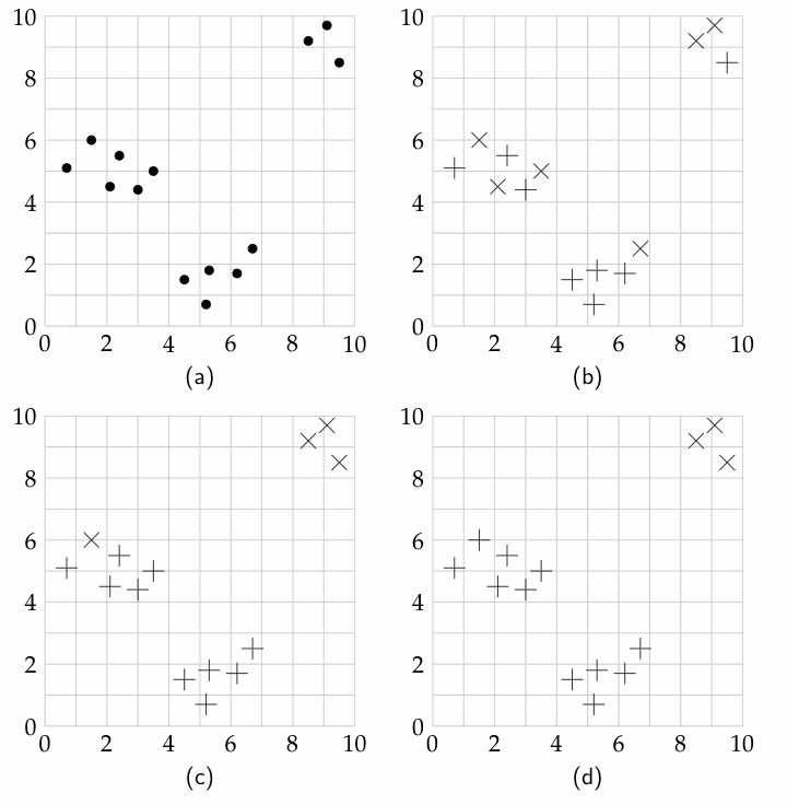
These data points are plotted in part (a) of Figure 11.1. Suppose the agent wants to cluster the data points into two classes.

In part (b), the points are randomly assigned into the classes; one class is depicted as + and the other as ×. The mean of the points marked with + is ⟨4.6,3.65⟩. The mean of the points marked with × is ⟨5.2,6.15⟩.
In part (c), the points are reassigned according to the closer of the two means. After this reassignment, the mean of the points marked with + is then ⟨3.96,3.27⟩. The mean of the points marked with × is ⟨7.15,8.34⟩.
In part (d), the points are reassigned to the closest mean. This assignment is stable in that no further reassignment will change the assignment of the examples.
A different initial assignment to the points can give different clustering. One clustering that arises in this data set is for the lower points (those with a Y-value less than 3) to be in one class, and for the other points to be in another class.
Running the algorithm with three classes would separate the data into the top-right cluster, the left-center cluster, and the lower cluster.
One problem with the k-means algorithm is the relative scale of the dimensions. For example, if one feature is height, another feature is age, and another is a binary feature, you must scale the different domains so that they can be compared. How they are scaled relative to each other affects the classification.
To find an appropriate number of classes, an agent can search over the number of classes. Note that k+1 classes can always result in a lower error than k classes as long as more than k different values are involved. A natural number of classes would be a value k when there is a large reduction in error going from k-1 classes to k classes, but in which there is only gradual reduction in error for larger values. Note that the optimal division into three classes, for example, may be quite different from the optimal division into two classes.


