Third edition of Artificial Intelligence: foundations of computational agents, Cambridge University Press, 2023 is now available (including the full text).
7.4.1 Neural Networks
Neural networks are a popular target representation for learning. These networks are inspired by the neurons in the brain but do not actually simulate neurons. Artificial neural networks typically contain many fewer than the approximately 1011 neurons that are in the human brain, and the artificial neurons, called units, are much simpler than their biological counterparts.
Artificial neural networks are interesting to study for a number of reasons:
- As part of neuroscience, to understand real neural systems, researchers are simulating the neural systems of simple animals such as worms, which promises to lead to an understanding about which aspects of neural systems are necessary to explain the behavior of these animals.
- Some researchers seek to automate not only the functionality of intelligence (which is what the field of artificial intelligence is about) but also the mechanism of the brain, suitably abstracted. One hypothesis is that the only way to build the functionality of the brain is by using the mechanism of the brain. This hypothesis can be tested by attempting to build intelligence using the mechanism of the brain, as well as without using the mechanism of the brain. Experience with building other machines - such as flying machines, which use the same principles, but not the same mechanism, that birds use to fly - would indicate that this hypothesis may not be true. However, it is interesting to test the hypothesis.
- The brain inspires a new way to think about computation that contrasts with currently available computers. Unlike current computers, which have a few processors and a large but essentially inert memory, the brain consists of a huge number of asynchronous distributed processes, all running concurrently with no master controller. One should not think that the current computers are the only architecture available for computation.
- As far as learning is concerned, neural networks provide a different measure of simplicity as a learning bias than, for example, decision trees. Multilayer neural networks, like decision trees, can represent any function of a set of discrete features. However, the functions that correspond to simple neural networks do not necessarily correspond to simple decision trees. Neural network learning imposes a different bias than decision tree learning. Which is better, in practice, is an empirical question that can be tested on different domains.
There are many different types of neural networks. This book considers one kind of neural network, the feed-forward neural network. Feed-forward networks can be seen as cascaded squashed linear functions. The inputs feed into a layer of hidden units, which can feed into layers of more hidden units, which eventually feed into the output layer. Each of the hidden units is a squashed linear function of its inputs.
Neural networks of this type can have as inputs any real numbers, and they have a real number as output. For regression, it is typical for the output units to be a linear function of their inputs. For classification it is typical for the output to be a sigmoid function of its inputs (because there is no point in predicting a value outside of [0,1]). For the hidden layers, there is no point in having their output be a linear function of their inputs because a linear function of a linear function is a linear function; adding the extra layers gives no added functionality. The output of each hidden unit is thus a squashed linear function of its inputs.
Associated with a network are the parameters for all of the linear functions. These parameters can be tuned simultaneously to minimize the prediction error on the training examples.
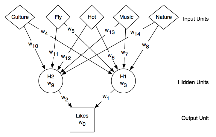
pval(e,Likes) = f(w0+w1×val(e,H1)+w2×val(e,H2)) val(e,H1) = f(w3+w4×val(e,Culture)+w5×val(e,Fly) +w6×val(e,Hot)+ w7×val(e,Music)+ w8×val(e,Nature) val(e,H2) = f(w9+w10×val(e,Culture)+w11×val(e,Fly) +w12×val(e,Hot)+ w13×val(e,Music) + w14×val(e,Nature)) ,
where f(x) is an activation function. For this example, there are 15 real numbers to be learned (w0,...,w14). The hypothesis space is thus a 15-dimensional real space. Each point in this 15-dimensional space corresponds to a function that predicts a value for Likes for every example with Culture, Fly, Hot, Music, and Nature given.
Given particular values for the parameters, and given values for the inputs, a neural network predicts a value for each target feature. The aim of neural network learning is, given a set of examples, to find parameter settings that minimize the error. If there are m parameters, finding the parameter settings with minimum error involves searching through an m-dimensional Euclidean space.
Back-propagation learning is gradient descent search through the parameter space to minimize the sum-of-squares error.
2: Inputs
3: X: set of input features, X={X1,...,Xn}
4: Y: set of target features, Y={Y1,...,Yk}
5: E: set of examples from which to learn
6: nh: number of hidden units
7: η: learning rate
8: Output
9: hidden unit weights hw[0:n,1:nh]
10: output unit weights ow[0:nh,1:k]
11: Local
12: hw[0:n,1:nh] weights for hidden units
13: ow[0:nh,1:k] weights for output units
14: hid[0:nh] values for hidden units
15: hErr[1:nh] errors for hidden units
16: out[1:k] predicted values for output units
17: oErr[1:k] errors for output units
18: initialize hw and ow randomly
19: hid[0]←1
20: repeat
21: for each example e in E do
22: for each h ∈{1,...,nh} do
23: hid[h] ← f(∑i=0n hw[i,h] ×val(e,Xi))
24: for each o ∈{1,...,k} do
25: out[o] ← f(∑h=0n hw[i,h] ×hid[h])
26: oErr[o] ←out[o]×(1-out[o])×(val(e,Yo)-out[o])
27: for each h ∈{0,...,nh} do
28: hErr[h] ←hid[h]×(1-hid[h])×∑o=0k ow[h,o] ×oErr[o]
29: for each i ∈{0,...,n} do
30: hw[i,h]←hw[i,h] + η×hErr[h]×val(e,Xi)
31: for each o ∈{1,...,k} do
32: ow[h,o]←ow[h,o] + η×oErr[o]×hid[h]
33: until termination
34: return w0,...,wn
Figure 7.12 gives the incremental gradient descent version of back-propagation for networks with one layer of hidden units. This approach assumes n input features, k output features, and nh hidden units. Both hw and ow are two-dimensional arrays of weights. Note that 0:nk means the index ranges from 0 to nk (inclusive) and 1:nk means the index ranges from 1 to nk (inclusive). This algorithm assumes that val(e,X0)=1 for all e.
The back-propagation algorithm is similar to the linear learner of Figure 7.6, but it takes into account multiple layers and the activation function. Intuitively, for each example it involves simulating the network on that example, determining first the value of the hidden units (line 25) then the value of the output units (line 28). It then passes the error back through the network, computing the error on the output nodes (line 29) and the error on the hidden nodes (line 32). It then updates all of the weights based on the derivative of the error.
Gradient descent search involves repeated evaluation of the function to be minimized - in this case the error - and its derivative. An evaluation of the error involves iterating through all of the examples. Back-propagation learning thus involves repeatedly evaluating the network on all examples. Fortunately, with the logistic function the derivative is easy to determine given the value of the output for each unit.
H1=f( -2.0×Culture -4.43×Fly+ 2.5×Hot +2.4×Music-6.1×Nature+1.63) H2=f( -0.7×Culture +3.0×Fly+ 5.8×Hot +2.0×Music-1.7×Nature-5.0) Likes=f( -8.5×H1 -8.8×H2 + 4.36) .
The use of neural networks may seem to challenge the physical symbol system hypothesis, which relies on symbols having meaning. Part of the appeal of neural networks is that, although meaning is attached to the input and output units, the designer does not associate a meaning with the hidden units. What the hidden units actually represent is something that is learned. After a neural network has been trained, it is often possible to look inside the network to determine what a particular hidden unit actually represents. Sometimes it is easy to express concisely in language what it represents, but often it is not. However, arguably, the computer has an internal meaning; it can explain its internal meaning by showing how examples map into the values of the hidden unit.
