Third edition of Artificial Intelligence: foundations of computational agents, Cambridge University Press, 2023 is now available (including the full text).
4.10.2.1 Continuous Domains
For optimization where the domains are continuous, a local search becomes more complicated because it is not obvious what the neighbors of a total assignment are. This problem does not arise with hard constraint satisfaction problems because the constraints implicitly discretize the space.
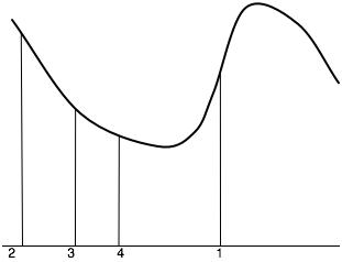
For optimization, gradient descent can be used to find a minimum value, and gradient ascent can be used to find a maximum value. Gradient descent is like walking downhill and always taking a step in the direction that goes down the most. The general idea is that the neighbor of a total assignment is to step downhill in proportion to the slope of the evaluation function h. Thus, gradient descent takes steps in each direction proportional to the negative of the partial derivative in that direction.
In one dimension, if X is a real-valued variable with the current value of v, the next value should be
v-η×(dh/dX)(v),
where
- η, the step size, is the constant of proportionality that determines how fast gradient descent approaches the minimum. If η is too large, the algorithm can overshoot the minimum; if η is too small, progress becomes very slow.
- (d h)/(d X), the derivative of h with respect to X, is a function of X and is evaluated for X=v.
For multidimensional optimization, when there are many variables, gradient descent takes a step in each dimension proportional to the partial derivative of that dimension. If ⟨X1,..., Xn⟩ are the variables that have to be assigned values, a total assignment corresponds to a tuple of values ⟨v1,..., vn⟩. Assume that the evaluation function, h, is differentiable. The next neighbor of the total assignment ⟨v1,..., vn⟩ is obtained by moving in each direction in proportion to the slope of h in that direction. The new value for Xi is
vi - η×(∂h /∂Xi)(v1,..., vn),
where η is the step size. The partial derivative, (∂h /∂Xi), is a function of X1,...,Xn. Applying it to the point (v1,..., vn) gives
(∂h /∂Xi)(v1,..., vn) = limε→∞ (h(v1,...,vi+ε,..., vn)- h(v1,...,vi,..., vn))/ε.
If the partial derivative of h can be computed analytically, it is usually good to do so. If not, it can be estimated using a small value of ε.
Gradient descent is used for parameter learning, in which there may be thousands of real-valued parameters to be optimized. There are many variants of this algorithm that we do not discuss. For example, instead of using a constant step size, the algorithm could do a binary search to determine a locally optimal step size.
