Third edition of Artificial Intelligence: foundations of computational agents, Cambridge University Press, 2023 is now available (including the full text).
7.3.2.1 Squashed Linear Functions
The use of a linear function does not work well for classification tasks. When there are only two values, say 0 and 1, a learner should never make a prediction of greater than 1 or less than 0. However, a linear function could make a prediction of, say, 3 for one example just to fit other examples better.
Initially let's consider binary classification, where the domain of the target variable is {0,1}. If multiple binary target variables exist, they can be learned separately.
For classification, we often use a squashed linear function of the form
fw(X1,...,Xn) = f( w0+w1 ×X1 + ...+ wn ×Xn) ,
where f is an activation function, which is a function from real numbers into [0,1]. Using a squashed linear function to predict a value for the target feature means that the prediction for example e for target feature Y is
pvalw(e,Y)=f(w0+w1 ×val(e,X1) + ...+ wn ×val(e,Xn)) .
A simple activation function is the step function, f(x), defined by
f(x)=
1 if x ≥ 0 0 if x< 0 .
A step function was the basis for the perceptron [Rosenblatt (1958)], which was one of the first methods developed for learning. It is difficult to adapt gradient descent to step functions because gradient descent takes derivatives and step functions are not differentiable.
If the activation is differentiable, we can use gradient descent to update the weights. The sum-of-squares error is
ErrorE(w) = ∑e∈E (val(e,Y)-f(∑i wi ×val(e,Xi)))2.
The partial derivative with respect to weight wi for example e is
∂ErrorE(w)/∂wi=-2×δ×f'(∑i wi ×val(e,Xi)) ×val(e,Xi) .
where δ=val(e,Y)-pvalw(e,Y), as before. Thus, each example e updates each weight wi as follows:
wi ← wi+η×δ×f'(∑i wi ×val(e,Xi)) ×val(e,Xi) .
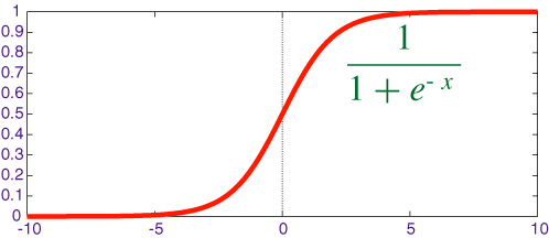
A typical differentiable activation function is the sigmoid or logistic function:
f(x)= 1/(1+e-x) .
This function, depicted in Figure 7.7, squashes the real line into the interval (0,1), which is appropriate for classification because we would never want to make a prediction of greater than 1 or less than 0. It is also differentiable, with a simple derivative - namely, f'(x)=f(x)×(1-f(x)) - which can be computed using just the values of the outputs.
The Linear Learner algorithm of Figure 7.6 can be changed to use the sigmoid function by changing line 17 to
wi←wi+η×δ×pvalw(e,Y)×[1-pvalw(e,Y)] ×val(e,Xi) .
where pvalw(e,Y)=f(∑i wi ×val(e,Xi)) is the predicted value of feature Y for example e.
Reads = f(-8+7×Short + 3 ×New + 3 ×Known) ,
where f is the sigmoid function. A function similar to this can be found with about 3,000 iterations of gradient descent with a learning rate η=0.05. According to this function, Reads is true (the predicted value is closer to 1 than 0) if and only if Short is true and either New or Known is true. Thus, the linear classifier learns the same function as the decision tree learner. To see how this works, see the "mail reading" example of the Neural AISpace.org applet.
This algorithm with the sigmoid function as the activation function can learn any linearly separable classification in the sense that the error can be made arbitrarily small on arbitrary sets of examples if, and only if, the target classification is linearly separable. A classification is linearly separable if there exists a hyperplane where the classification is true on one side of the hyperplane and false on the other side. The hyperplane is defined as where the predicted value, fw(X1,...,Xn) = f(w0+w1 ×val(e,X1) + ...+ wn ×val(e,Xn)), is 0.5. For the sigmoid activation function, this occurs when w0+w1 ×val(e,X1) + ...+ wn ×val(e,Xn)=0 for the learned weights w. On one side of this hyperplane, the prediction is greater than 0.5; on the other side, it is less than 0.5.
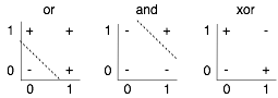
Figure 7.8 shows linear separators for "or" and "and". The dashed line separates the positive (true) cases from the negative (false) cases. One simple function that is not linearly separable is the exclusive-or (xor) function, shown on the right. There is no straight line that separates the positive examples from the negative examples. As a result, a linear classifier cannot represent, and therefore cannot learn, the exclusive-or function.
Often it is difficult to determine a priori whether a data set is linearly separable.
| Culture | Fly | Hot | Music | Nature | Likes |
| 0 | 0 | 1 | 0 | 0 | 0 |
| 0 | 1 | 1 | 0 | 0 | 0 |
| 1 | 1 | 1 | 1 | 1 | 0 |
| 0 | 1 | 1 | 1 | 1 | 0 |
| 0 | 1 | 1 | 0 | 1 | 0 |
| 1 | 0 | 0 | 1 | 1 | 1 |
| 0 | 0 | 0 | 0 | 0 | 0 |
| 0 | 0 | 0 | 1 | 1 | 1 |
| 1 | 1 | 1 | 0 | 0 | 0 |
| 1 | 1 | 0 | 1 | 1 | 1 |
| 1 | 1 | 0 | 0 | 0 | 1 |
| 1 | 0 | 1 | 0 | 1 | 1 |
| 0 | 0 | 0 | 1 | 0 | 0 |
| 1 | 0 | 1 | 1 | 0 | 0 |
| 1 | 1 | 1 | 1 | 0 | 0 |
| 1 | 0 | 0 | 1 | 0 | 0 |
| 1 | 1 | 1 | 0 | 1 | 0 |
| 0 | 0 | 0 | 0 | 1 | 1 |
| 0 | 1 | 0 | 0 | 0 | 1 |
After 10,000 iterations of gradient descent with a learning rate of 0.05, the optimal prediction is (to one decimal point)
Likes=f( 2.3×Culture +0.01×Fly-9.1×Hot -4.5×Music+6.8×Nature+0.01) ,
which approximately predicts the target value for all of the tuples in the training set except for the last and the third-to-last tuple, for which it predicts a value of about 0.5. This function seems to be quite stable with different initializations. Increasing the number of iterations makes it predict the other tuples better.
When the domain of the target variable is greater than 2 - there are more than two classes - indicator variables can be used to convert the classification to binary variables. These binary variables could be learned separately. However, the outputs of the individual classifiers must be combined to give a prediction for the target variable. Because exactly one of the values must be true for each example, the learner should not predict that more than one will be true or that none will be true. A classifier that predicts a probability distribution can normalize the predictions of the individual predictions. A learner that must make a definitive prediction can use the mode.
