Artificial
Intelligence 2E
foundations of computational agents
The third edition of Artificial Intelligence: foundations of computational agents, Cambridge University Press, 2023 is now available (including full text).
8.9 Exercises
-
1.
Bickel et al. [1975] report on gender biases for graduate admissions at UC Berkeley. This example is based on that case, but the numbers are fictional.
There are two departments, which we will call and (so is a random variable with values and ) which students can apply to. Assume students apply to one, but not both. Students have a gender (male or female), and are either admitted or not. Consider the table of the percent of students in each category of Figure 8.33.
Dept Gender Admitted Percent 32 18 7 3 5 14 7 14 Figure 8.33: Counts for students in departments In the semantics of possible worlds, we will treat the students as possible worlds, each with the same measure.
-
(a)
What is ?
What is ?
Which gender is more likely to be admitted? -
(b)
What is ?
What is ?
Which gender is more likely to be admitted to ? -
(c)
What is ?
What is ?
Which gender is more likely to be admitted to ? -
(d)
This is an instance of Simpson’s paradox. Why is it a paradox? Explain why it happened in this case.
-
(e)
Give another scenario where Simpson’s paradox occurs.
-
(a)
-
2.
Prove Proposition 8.1 for finitely many worlds, namely that the axioms of probability (Section 8.1.2) are sound and complete with respect to the semantics of probability. [Hint: For soundness, show that each of the axioms is true based on the semantics. For completeness, construct a probability measure from the axioms.]
-
3.
Using only the axioms of probability and the definition of conditional independence, prove Proposition 8.5.
-
4.
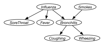
Figure 8.34: A simple diagnostic belief network Consider the belief network of Figure 8.34. This the “Simple diagnostic example” in the AIspace belief network tool at http://www.aispace.org/bayes/. For each of the following, first predict the answer based on your intuition, then run the belief network to check it. Explain the result you found by carrying out the inference.
-
(a)
The posterior probabilities of which variables change when is observed to be true? That is, give the variables such that .
-
(b)
Starting from the original network, the posterior probabilities of which variables change when is observed to be true? That is, specify the where .
-
(c)
Does the probability of change when is observed to be true?
That is, is ? Explain why (in terms of the domain, in language that could be understood by someone who did not know about belief networks). -
(d)
Suppose is observed to be true. Does the observing change the probability of ? That is, is ? Explain why (in terms that could be understood by someone who did not know about belief networks).
-
(e)
What could be observed so that subsequently observing does not change the probability of . That is, specify a variable or variables such that , or state that there are none. Explain why.
-
(f)
Suppose could be another explanation of . Change the network so that also affects but is independent of the other variables in the network. Give reasonable probabilities.
-
(g)
What could be observed so that observing changes the probability of ? Explain why.
-
(h)
What could be observed so that observing changes the probability of ? Explain why.
Note that parts (a), (b), and (c) only involve observing a single variable.
-
(a)
-
5.
Consider the belief network of Figure 8.35, which extends the electrical domain to include an overhead projector.
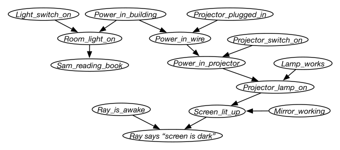
Figure 8.35: Belief network for an overhead projector Answer the following questions about how knowledge of the values of some variables would affect the probability of another variable.
-
(a)
Can knowledge of the value of affect your belief in the value of ? Explain.
-
(b)
Can knowledge of affect your belief in ? Explain.
-
(c)
Can knowledge of affect your belief in given that you have observed a value for ? Explain.
-
(d)
Which variables could have their probabilities changed if just was observed?
-
(e)
Which variables could have their probabilities changed if just was observed?
-
(a)
-
6.
Kahneman [2011, p. 166] gives the following example.
A cab was involved in a hit-and-run accident at night. Two cab companies, Green and Blue, operate in the city. You are given the following data:
-
•
85% of the cabs in the city are Green and 15% are Blue.
-
•
A witness identified the cab as Blue. The court tested the reliability of the witness in the circumstances that existed on the night of the accident and concluded that the witness correctly identifies each one of the two colors 80% of the time and fails 20% of the time.
What is the probability that the cab involved in the accident was Blue?
-
(a)
Represent this story as a belief network. Explain all variables and conditional probabilities. What is observed, what is the answer?
-
(b)
Suppose there were three independent witnesses, two of which claimed the cab was Blue and one of whom claimed the cab was Green. Show the corresponding belief network. What is the probability the cab was Blue? What if all three claimed the cab was Blue?
-
(c)
Suppose it was found that the two witnesses who claimed the cab was Blue were not independent, but there was a 60% chance they colluded. (What might this mean?) Show the corresponding belief network, and the relevant probabilities. What is the probability that the cab is Blue, (both for the case where all three witnesses claim that cab was Blue and the case where the other witness claimed the cab was Green)?
-
(d)
In a variant of this scenario, Kahneman [2011, p. 167] replaced the first condition with: “The two companies operate the same number of cabs, but Green cabs are involved in 85% of the accidents.” How can this new scenario be represented as a belief network? Your belief network should allow observations about whether there is an accident as well as the color of the taxi. Show examples of inferences in your network. Make reasonable choices for anything that is not fully specified. Be explicit about any assumptions you make.
-
•
-
7.
Represent the same scenario as in Exercise 8 using a belief network. Show the network structure. Give all of the initial factors, making reasonable assumptions about the conditional probabilities (they should follow the story given in that exercise, but allow some noise). Give a qualitative explanation of why the patient has spots and fever.
-
8.
Suppose you want to diagnose the errors school students make when adding multidigit binary numbers. Consider adding two two-digit numbers to form a three-digit number.
That is, the problem is of the form:
where , , and are all binary digits.
-
(a)
Suppose you want to model whether students know binary addition and whether they know how to carry. If students know how, they usually get the correct answer, but sometimes make mistakes. Students who do not know how to do the appropriate task simply guess.
What variables are necessary to model binary addition and the errors students could make? You must specify, in words, what each of the variables represents. Give a DAG that specifies the dependence of these variables.
-
(b)
What are reasonable conditional probabilities for this domain?
-
(c)
Implement this, perhaps by using the AIspace.org belief-network tool. Test your representation on a number of different cases.
You must give the graph, explain what each variable means, give the probability tables, and show how it works on a number of examples.
-
(a)
-
9.
In this question, you will build a belief network representation of the Deep Space 1 (DS1) spacecraft considered in Exercise 10. Figure 5.14 depicts a part of the actual DS1 engine design.
Consider the following scenario.
-
•
Valves are or .
-
•
A value can be , in which case the gas will flow if the valve is open and not if it is closed; , in which case gas never flows; , in which case gas flows independently of whether the valve is open or closed; or , in which case gas flowing into the valve leaks out instead of flowing through.
-
•
There are three gas sensors that can detect whether gas is leaking (but not which gas); the first gas sensor detects gas from the rightmost valves (), the second gas sensor detects gas from the center valves (), and the third gas sensor detects gas from the leftmost valves ().
-
(a)
Build a belief-network representation of the domain. You only must consider the topmost valves (those that feed into engine ). Make sure there are appropriate probabilities.
-
(b)
Test your model on some non-trivial examples.
-
•
-
10.
Consider the following belief network:
with Boolean variables (we write as and as ) and the following conditional probabilities:
-
(a)
Compute using variable elimination (VE). You should first prune irrelevant variables. Show the factors that are created for a given elimination ordering.
-
(b)
Suppose you want to compute using VE. How much of the previous computation is reusable? Show the factors that are different from those in part (a).
-
(a)
-
11.
Explain how to extend VE to allow for more general observations and queries. In particular, answer the following.
-
(a)
How can the VE algorithm be extended to allow observations that are disjunctions of values for a variable (e.g., of the form )?
-
(b)
How can the VE algorithm be extended to allow observations that are disjunctions of values for different variables (e.g., of the form )?
-
(c)
How can the VE algorithm be extended to allow for the probability on a set of variables (e.g., asking for the )?
-
(a)
-
12.
In a nuclear research submarine, a sensor measures the temperature of the reactor core. An alarm is triggered () if the sensor reading is abnormally high (), indicating an overheating of the core (). The alarm and/or the sensor could be defective (, ), which causes them to malfunction. The alarm system is modeled by the belief network of Figure 8.36.
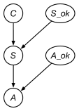
Figure 8.36: Belief network for a nuclear submarine -
(a)
What are the initial factors for this network? For each factor, state what it represents and what variables it is a function of.
-
(b)
Show how VE can be used to compute the probability that the core is overheating, given that the alarm does not go off; that is, . For each variable eliminated, show which variable is eliminated, which factor(s) are removed, and which factor(s) are created, including what variables each factor is a function of. Explain how the answer is derived from the final factor.
-
(c)
Suppose we add a second, identical sensor to the system and trigger the alarm when either of the sensors reads a high temperature. The two sensors break and fail independently. Give the corresponding extended belief network.
-
(a)
-
13.
In this exercise, we continue Exercise 14.
-
(a)
Explain what knowledge (about physics and about students) a belief-network model requires.
-
(b)
What is the main advantage of using belief networks over using abductive diagnosis or consistency-based diagnosis in this domain?
-
(c)
What is the main advantage of using abductive diagnosis or consistency-based diagnosis over using belief networks in this domain?
-
(a)
-
14.
Suppose Kim has a camper van (a mobile home) and likes to keep it at a comfortable temperature and noticed that the energy use depended on the elevation. Kim knows that the elevation affects the outside temperature. Kim likes the camper warmer at higher elevation. Note that not all of the variables directly affect electrical usage.
-
(a)
Show how this can be represented as a causal network, using the variables “Elevation”, “Electrical Usage”, “Outside Temperature”, “Thermostat Setting”.
-
(b)
Give an example where intervening has an effect different from conditioning for this network.
-
(a)
-
15.
The aim of this exercise is to extend Example 8.29. Suppose the animal is either sleeping, foraging or agitated.
If the animal is sleeping at any time, it does not make a noise, does not move and at the next time point it is sleeping with probability 0.8 or foraging or agitated with probability 0.1 each.
If the animal is foraging or agitated, it tends to remain in the same state of composure (with probability 0.8) move to the other state of composure with probability 0.1 or go to sleep with probability 0.1.
If the animal is foraging in a corner, it will be detected by the microphone at that corner with probability 0.5, and if the animal is agitated in a corner it will be detected by the microphone at that corner with probability 0.9. If the animal is foraging in the middle, it will be detected by each of the microphones with probability 0.2. If it is agitated in the middle it will be detected by each of the microphones with probability 0.6. Otherwise the microphones have a false positive rate of 0.05.
-
(a)
Represent this as a two-stage dynamic belief network. Draw the network, give the domains of the variables and the conditional probabilities.
-
(b)
What independence assumptions are embedded in the network?
-
(c)
Implement either variable elimination or particle filtering for this problem.
-
(d)
Does being able to hypothesize the internal state of the agent (whether it is sleeping, foraging, or agitated) help localization? Explain why.
-
(a)
-
16.
Suppose Sam built a robot with five sensors and wanted to keep track of the location of the robot, and built a hidden Markov model (HMM) with the following structure (which repeats to the right):
-
(a)
What probabilities does Sam need to provide? You should label a copy of the diagram, if that helps explain your answer.
-
(b)
What independence assumptions are made in this model?
-
(c)
Sam discovered that the HMM with five sensors did not work as well as a version that only used two sensors. Explain why this may have occurred.
-
(a)
-
17.
Consider the problem of filtering in HMMs.
-
(a)
Give a formula for the probability of some variable given future and past observations. You can base this on Equation 8.2. This should involve obtaining a factor from the previous state and a factor from the next state and combining them to determine the posterior probability of . [Hint: Consider how VE, eliminating from the leftmost variable and eliminating from the rightmost variable, can be used to compute the posterior distribution for .]
-
(b)
Computing the probability of all of the variables can be done in time linear in the number of variables by not recomputing values that were already computed for other variables. Give an algorithm for this.
-
(c)
Suppose you have computed the probability distribution for each state …, , and then you get an observation for time . How can the posterior probability of each variable be updated in time linear in ? [Hint: You may need to store more than just the distribution over each .]
-
(a)
-
18.
Which of the following algorithms suffers from underflow (real numbers that are too small to be represented using double precision floats): rejection sampling, importance sampling, particle filtering? Explain why. How could underflow be avoided?
-
19.
-
(a)
What are the independence assumptions made in the naive Bayes classifier for the help system of Example 8.35.
-
(b)
Are these independence assumptions reasonable? Explain why or why not.
-
(c)
Suppose we have a topic-model network like the one of Figure 8.26, but where all of the topics are parents of all of the words. What are all of the independencies of this model?
-
(d)
Give an example where the topics would not be independent.
-
(a)
-
20.
Suppose you get a job where the boss is interested in localization of a robot that is carrying a camera around a factory. The boss has heard of variable elimination, rejection sampling, and particle filtering and wants to know which would be most suitable for this task. You must write a report for your boss (using proper English sentences), explaining which one of these technologies would be most suitable. For the two technologies that are not the most suitable, explain why you rejected them. For the one that is most suitable, explain what information is required by that technology to use it for localization:
-
(a)
VE (i.e., exact inference as used in HMMs),
-
(b)
rejection sampling, or
-
(c)
particle filtering.
-
(a)
-
21.
How well does particle filtering work for Example 8.46? Try to construct an example where Gibbs sampling works much better than particle filtering. [Hint: Consider unlikely observations after a sequence of variable assignments.]