15.3 Statistical Relational Artificial Intelligence 15.3 Statistical Relational Artificial Intelligence 15.4 Review

The third edition of Artificial Intelligence: foundations of computational agents, Cambridge University Press, 2023 is now available (including full text).

15.3.1 Relational Probabilistic Models

The belief network probability models of Chapter 8 were defined in terms of features. Many domains are best modeled in terms of individuals and relations. Agents must often build models before they know what individuals are in the domain and, therefore, before they know what random variables exist. When the probabilities are being learned, the probabilities often do not depend on the individuals. Although it is possible to learn about an individual, an agent must also learn general knowledge that it can apply when it finds out about a new individual.

$\begin{array}[]{c|c|c}Student&Course&Grade\\ \hline s_{1}&c_{1}&a\\ s_{2}&c_{1}&c\\ s_{1}&c_{2}&b\\ s_{2}&c_{3}&b\\ s_{3}&c_{2}&b\\ s_{4}&c_{3}&b\\ s_{3}&c_{4}&?\\ s_{4}&c_{4}&?\end{array}$

Figure 15.6: Predict which student will do better in course

c_{4}

Example 15.17.

Consider the problem of predicting how well students will do in courses they have not taken. Figure 15.6 shows some fictional data designed to show what can be done. Students $s_{3}$ and $s_{4}$ have the same averages, on courses with the same averages. However, we may be able to distinguish them as we know something about the courses they have taken.

This is a different problem than the cases consider in Chapter 7 because the values of properties $S t u d e n t$ and $C o u r s e$ are individuals, and we want to make predictions based on the properties of the individuals. None of the methods in that chapter would work on such data.

Example 15.18.

Consider the problem of an intelligent tutoring system diagnosing students’ arithmetic errors. From observing a student’s performance on a number of examples, the tutor should try to determine whether or not the student understands the task and, if not, work out what the student is doing wrong so that appropriate remedies can be applied.

Consider the case of diagnosing two-digit addition of the form

\begin{array}[b]{rrrr}&&x_{1}&x_{0}\\ +&&y_{1}&y_{0}\\ \hline&z_{2}&z_{1}&z_{0}\end{array}

The student is given the values for the $x$ s and the $y$ s and provides values for the $z$ s.

Students’ answers depend on the problem (the $x$ s and $y$ s) and whether they know basic addition and whether they know how to carry.

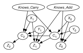
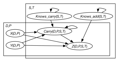
Figure 15.7: Belief network for two-digit addition

A belief network for this example is shown in Figure 15.7. The carry into digit $i$ , given by the variable $C_{i}$ , depends on the $X_{i}$ , $Y_{i}$ , and $C_{i-1}$ , the carry for the previous digit (except for the initial case), and on whether the student knows how to carry. The $z$ -value for digit $i$ , given by the variable $Z_{i}$ , depends on the $X_{i}$ , $Y_{i}$ , $C_{i}$ , and whether the student knows basic addition.

By observing the value of the $x$ s and the $y$ s in the problem and the value of $z$ s given by the student, the posterior probability that the student knows addition and knows how to carry can be inferred. One feature of the belief network model is that it allows students to make random errors; even though they know how to perform two-digit arithmetic, they can still get the wrong answer occasionally.

The problem with this representation is that it is inflexible. A flexible representation would allow for the addition of multiple digits, multiple problems, multiple students, and multiple times. Multiple digits require the replication of the network for the digits. Multiple times allow for modeling how students’ knowledge and their answers change over time, even if the problems do not change over time.

If the conditional probabilities were stored as tables, the size of those tables would be enormous. For example, if the $X_{i}$ , $Y_{i}$ , and $Z_{i}$ variables each have a domain size of 11 (the digits 0 to 9 or the blank), and the $C_{i}$ and $Knows\_Add$ variables are binary, a tabular representation of

P(Z_{1}|X_{1},Y_{1},C_{1},Knows\_Add)

would have a size greater than 4000. There is much more structure in the conditional probability than is expressed in the tabular representation. Tabular representations are not the only representation of conditional probabilities. We present a probabilistic extension of logic programs below that allows for both relational probabilistic models and compact descriptions of conditional probabilities.

A relational probability model (RPM) or probabilistic relational model is a model in which the probabilities are specified on the relations, independently of the actual individuals. Different individuals share the probability parameters.

A parameterized random variable is of the form $R(t_{1},\ldots,t_{n})$ , where each $t_{i}$ is a term (a logical variable or a constant). Thus it corresponds to either an atomic symbol or a term. The parameterized random variable is said to be parameterized by the logical variables that appear in it. A ground instance of a parameterized random variable is obtained by substituting constants for the logical variables in the parameterized random variable. The ground instances of a parameterized random variable correspond to random variables. The domain of the random variable is the range of $R$ . A Boolean parameterized random variable $R$ corresponds to a predicate symbol.

We use the Datalog convention that logical variables start with an upper-case letter and constants start with a lower-case letter. Random variables and functions are written starting with an upper-case letter, with the corresponding proposition in lower case (e.g., $Diff(c_{1}){=}true$ is written as $diff(c_{1})$ , and $Diff(c_{1}){=}false$ is written as $\neg diff(c_{1})$ ).

Example 15.19.

For a relational probability model of the multidigit arithmetic problem outlined above, there is a separate $x$ -variable for each digit $D$ and for each problem $P$ , represented by the parameterized random variable $X(D,P)$ . Thus, for example, $X(1,prob17)$ may be a random variable representing the $x$ -value of the first digit of problem 17. Similarly there is a parameterized random variable, $Y(D,P)$ , which represents a random variable for each digit $D$ and problem $P$ .

There is a variable for each student $S$ and time $T$ that represents whether $S$ knows how to add properly at time $T$ . The parameterized random variable $Knows\_add(S,T)$ represents whether student $S$ knows addition at time $T$ . The random variable $Knows\_add(fred,mar23)$ is true if Fred knows addition on March 23. Similarly, there is a parameterized random variable $Knows\_carry(S,T)$ .

There is a different $z$ -value and a different carry for each digit, problem, student, and time. These values are represented by the parameterized random variables $Z(D,P,S,T)$ and $Carry(D,P,S,T)$ . So, $Z(1,prob17,fred,mar23)$ is a random variable representing the answer Fred gave on March 23 for digit 1 of problem 17. Function $Z$ has range $\{0,\dots,9,blank\}$ , so this set is the domain of the random variables that are the ground instances of $Z(D,P,S,T)$ .

A plate model consists of

•

a directed graph in which the nodes are parameterized random variables,
•

a population of individuals for each logical variable, and
•

a conditional probability of each node given its parents.

We draw a rectangle – a plate – around the parameterized random variables that share a logical variable. There is a plate for each logical variable. A plate model means its grounding – the belief network in which nodes are all ground instances of the parameterized random variables (each logical variable replaced by an individual in its population). That is, the variables in each plate are replicated for each individual. The conditional probabilities of the grounded belief network are the same as the corresponding instances of the plate model. This notation is redundant, as the logical variables are specified in both the plates and the arguments. Sometimes one of these is omitted; often the arguments are omitted when they can be inferred from the plates.

Figure 15.8: A plate model to predict the grades of students

Example 15.20.

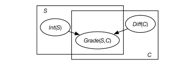
Figure 15.8 gives a plate model for predicting student grades. There is a plate $C$ for the courses and a plate $S$ for the students. The parameterized random variables are

•

$Int(S)$ which represents whether student $S$ is intelligent
•

$DiffC)$ , which represents whether course $C$ is difficult,
•

$Grade(S,C)$ which represents the grade of student $S$ in course $C$ .

The probabilities for $P(Int(S))$ , $P(DiffC))$ , and $P(Grade(S,C)\mid Int(S),DiffC))$ need to be specified. If $I$ and $D$ are Boolean (with range $t r u e$ and $f a l s e$ ) and $G r$ has range $\{a,b,c\}$ then there are 10 parameters that define the probability distribution. Suppose $P(Int(S))=0.5$ and $P(DiffC))=0.5$ and $P(Grade(S,C)\mid Int(S),DiffC))$ is defined by the following table:

\begin{array}[b]{ll|lll}Int(S)&DiffC)&\omit\span\omit\span\omit Grade(S,C)\\ &&a&b&c\\ \hline true&true&0.5&0.4&0.1\\ true&false&0.9&0.09&0.01\\ false&true&0.01&0.1&0.9\\ false&false&0.1&0.4&0.5\end{array}

Eight parameters are required to define $P(Grade(S,C)\mid Int(S),DiffC))$ because there are four cases, and each case requires two numbers to be specified; the third can be inferred to ensure the probabilities sum to one.

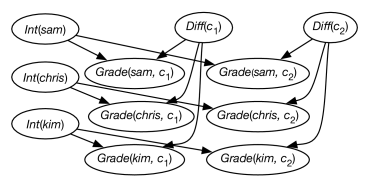
Figure 15.9: A grounding for 3 students and 2 courses

Figure 15.9 shows a grounding for 3 students $s a m$ , $c h r i s$ and $k i m$ , and 2 courses, $c_{1}$ and $c_{2}$ . If there were $n$ students and $m$ courses, in the grounding there would be $n$ instances of $Int(S)$ , $m$ instances of $DiffC)$ and $n*m$ instances of $Grade(S,C)$ . So there would be $n+m+n*m$ random variables in the grounding.

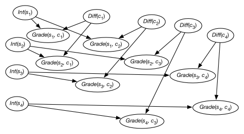
Consider conditioning on the data given in Figure 15.6, and querying the variables corresponding to the last two rows. There are 4 courses and 4 students, and so there would be 24 variables in the grounding. All of the instances of $Grade(S,C)$ that are not observed or queried can be pruned or never constructed in the first place, resulting in the belief network of Figure 15.10. From this network, conditioned on the $o b s$ , the observed grades of Figure 15.6, and using the probabilities above, the following posterior probabilities can be derived:

\begin{array}[b]{l|ccc}&a&b&c\\ \hline P(Grade(s_{3},c_{4})\mid obs)&0.491&0.245&0.264\\ P(Grade(s_{4},c_{4})\mid obs)&0.264&0.245&0.491\end{array}

Thus, this model predicts that $s_{3}$ is likely to do better than $s_{4}$ in course $c_{4}$ .

Figure 15.10: A grounding that is sufficient to predict from the data in Figure 15.6

Figure 15.11: Belief network with plates for multidigit addition

Example 15.21.

A plate model for the multidigit addition problem of Example 15.19 is shown in Figure 15.11. The rectangles correspond to plates. For the plate labeled with $D, P$ , an instance of each variable exists for each digit $D$ and problem $P$ . One way to view this is that the instances come out of the page, like a stack of plates. Similarly, for the plate labeled $S, T$ , there is a copy of the variables for each student $S$ and each time $T$ . For the variables in the intersection of the plates, there is a random variable for each digit $D$ , problem $P$ , student $S$ , and time $T$ .

The plate representation denotes the same independence as a belief network; each node is independent of its non-descendants given its parents. This dependence is inherited by a corresponding ground belief network. Thus, for particular values $d\in dom(D)$ , $p\in dom(P)$ , $s\in dom(S)$ , and $t\in dom(T)$ , $Z(d,p,s,t)$ is a random variable, with parents $X(d,p)$ , $Y(d,p)$ , $Carry(d,p,s,t)$ and $Knows\_add(s,t)$ . There is a loop in the plate model on the $Carry(D,P,S,T)$ parameterized random variable because the carry for one digit depends on the carry for the previous digit for the same problem, student, and time. Similarly, whether students know how to carry at some time depends on whether they knew how to carry at the previous time. The ground network needs to be acyclic.

There is a conditional probability of each parameterized random variable, given its parents. This conditional probability is shared among its ground instances.

Unfortunately, the plate representation is not adequate when the dependency occurs among different instances of the same relation. In the preceding example, $Carry(D,P,S,T)$ depends, in part, on $Carry(D-1,P,S,T)$ , that is, on the carry from the previous digit (and there is some other case for the first digit). To represent such examples, it is useful to be able to specify how the logical variables interact, as is done in logic programs.

One representation that combines the ideas of belief networks, plates, and logic programs is the independent choice logic (ICL). The ICL consists of a set of independent choices, a logic program that gives the consequences of the choices, and probability distributions over the choices. In more detail, the ICL is defined as follows:

An alternative is a set of atoms all sharing the same logical variables. A choice space is a set of alternatives such that none of the atoms in the alternatives unify with each other. An ICL theory contains

•

a choice space $C$ . Let $C^{\prime}$ be the set of ground instances of the alternatives. Thus, $C^{\prime}$ is a set of sets of ground atoms.
•

an acyclic logic program (that can include negation as failure), in which the head of the clauses does not unify with an element of an alternative in the choice space.
•

a probability distribution over each alternative. All instances of an alternative have the same probability.

The atoms in the logic program and the choice space can contain constants, variables, and function symbols.

A selector function selects a single element from each alternative in $C^{\prime}$ . There is a possible world for each selector function. The logic program specifies what is true in each possible world. Atom $g$ is true in a possible world if it follows from the atoms selected by the selector function added to the logic program. The probability of proposition $g$ is given by a measure over sets of possible worlds, where the atoms in different ground instances of the alternatives are probabilistically independent. The instances of an alternative share the same probabilities, and the probabilities of different instances are multiplied.

Example 15.22.

Consider the choice space $C=\{\{a_{1},a_{2}\},\{b_{1},b_{2},b_{3}\}\}$ , the logic program $L$ :

	$\displaystyle c$	$\displaystyle\leftarrow\mbox{}a_{1}\land b_{1}$
	$\displaystyle c$	$\displaystyle\leftarrow\mbox{}a_{2}\land b_{3}$
	$\displaystyle d$	$\displaystyle\leftarrow\mbox{}c$
	$\displaystyle d$	$\displaystyle\leftarrow\mbox{}b_{2}$

and the distribution over the first alternative, $P(a_{1})=0.7$ , $P(a_{2})=0.3$ and over the second alternative $P(b_{1})=0.5$ , $P(b_{2})=0.4$ , $P(b_{3})=0.1$ .

There are 6 possible worlds:

World	Selection		Implied by $L$		probability
$w_{0}$	$a_{1}$	$b_{1}$	$c$	$d$	0.35
$w_{1}$	$a_{1}$	$b_{2}$	$\neg c$	$d$	0.28
$w_{2}$	$a_{1}$	$b_{3}$	$\neg c$	$\neg d$	0.07
$w_{3}$	$a_{2}$	$b_{1}$	$\neg c$	$\neg d$	0.15
$w_{4}$	$a_{2}$	$b_{2}$	$\neg c$	$d$	0.12
$w_{5}$	$a_{2}$	$b_{3}$	$c$	$d$	0.03

so, under this model, $P(c)=0.35+0.03=0.38$ , and $P(d)=0.35+0.28+0.12+0.03=0.78$ .

You do not need to enumerate all possible worlds to compute probabilities. Abduction can be used to find descriptions of the sets of worlds in which $g$ is true. The atoms in the alternatives are made assumable, with different atoms in the same alternative declared to be inconsistent. If the explanations are pairwise inconsistent, the probability of $g$ can be computed by adding the probabilities of the explanations. If they are not pairwise inconsistent they can be made pairwise consistent.

An ICL theory can be seen as a causal model in which the causal mechanism is specified as a logic program and the background variables, corresponding to the alternatives, have independent probability distributions over them. It may seem that this logic, with only unconditionally independent atoms and a deterministic logic program, is too weak to represent the sort of knowledge required. However, even without logical variables, the independent choice logic can represent anything that can be represented in a belief network, as in the following example:

Example 15.23.

Consider representing the belief network of Example 8.15 in the ICL. The same technique works for any belief network.

Fire and tampering have no parents, so they can be represented directly as alternatives:

	$\displaystyle{\{fire,nofire\},}$
	$\displaystyle{\{tampering,notampering\}.}$

The probability distribution over the first alternative is $P(fire)=0.01$ , $P(nofire)=0.99$ . Similarly, $P(tampering)=0.02$ , $P(notampering)=0.89$ .

The dependence of $S m o k e$ on $F i r e$ can be represented using two alternatives:

	$\displaystyle{\{smokeWhenFire,nosmokeWhenFire\},}$
	$\displaystyle{\{smokeWhenNoFire,nosmokeWhenNoFire\},}$

with $P(smokeWhenFire)=0.9$ and $P(smokeWhenNoFire)=0.01$ . Two rules can be used to specify when there is smoke:

	$\displaystyle{smoke\leftarrow\mbox{}fire\wedge\mbox{}smokeWhenFire.}$
	$\displaystyle{smoke\leftarrow\mbox{}\mbox{$\sim$}fire\wedge\mbox{}% smokeWhenNoFire.}$

where $\sim$ is negation as failure, and so these clauses mean their completion.

To represent how $A l a r m$ depends on $F i r e$ and $T a m p e r i n g$ , there are four alternatives:

	$\displaystyle{\{alarmWhenTamperingFire,noalarmWhenTamperingFire\},}$
	$\displaystyle{\{alarmWhenNoTamperingFire,noalarmWhenNoTamperingFire\},}$
	$\displaystyle{\{alarmWhenTamperingNoFire,noalarmWhenTamperingNoFire\},}$
	$\displaystyle{\{alarmWhenNoTamperingNoFire,noalarmWhenNoTamperingNoFire\},}$

where $P(alarmWhenTamperingFire)=0.5$ , $P(alarmWhenNoTamperingFire)=0.99$ , and similarly for the other atoms using the probabilities from Example 8.15. There are also rules specifying when $a l a r m$ is true, depending on tampering and fire:

	$\displaystyle{alarm\leftarrow\mbox{}tampering\wedge\mbox{}fire\wedge\mbox{}% alarmWhenTamperingFire.}$
	$\displaystyle{alarm\leftarrow\mbox{}\mbox{$\sim$}tampering\wedge\mbox{}fire% \wedge\mbox{}alarmWhenNoTamperingFire.}$
	$\displaystyle{alarm\leftarrow\mbox{}tampering\wedge\mbox{}\mbox{$\sim$}fire% \wedge\mbox{}alarmWhenTamperingNoFire.}$
	$\displaystyle{alarm\leftarrow\mbox{}\mbox{$\sim$}tampering\wedge\mbox{}\mbox{$% \sim$}fire\wedge\mbox{}alarmWhenNoTamperingNoFire.}$

Other random variables are represented analogously, using the same number of alternatives as there are assignments of values to the parents of a node.

An ICL representation of a conditional probability can be seen as a rule form of a decision tree with probabilities at the leaves. There is a rule and an alternative for each branch. Non-binary alternatives are useful when non-binary variables are involved.

The independent choice logic may not seem very intuitive for representing standard belief networks, but it can make complicated relational models much simpler, as in the following example.

Example 15.24.

Consider the parameterized version of the multidigit addition of Example 15.19. The plates correspond to logical variables.

There are three cases for the value of $Z(D,P,S,T)$ . The first is when the student knows addition at this time, and the student did not make a mistake. In this case, they get the correct answer:

	$\displaystyle{z(D,P,S,T,V)\leftarrow\mbox{}}$
	$\displaystyle\ \ \ \ {x(D,P,Vx)\wedge\mbox{}}$
	$\displaystyle\ \ \ \ {y(D,P,Vy)\wedge\mbox{}}$
	$\displaystyle\ \ \ \ {carry(D,P,S,T,Vc)\wedge\mbox{}}$
	$\displaystyle\ \ \ \ {knowsAddition(S,T)\wedge\mbox{}}$
	$\displaystyle\ \ \ \ {\mbox{$\sim$}mistake(D,P,S,T)\wedge\mbox{}}$
	$\displaystyle\ \ \ \ {V\mbox{ is }(Vx+Vy+Vc)\mbox{ div }10.}$

We use the convention that the last variable in the atom corresponds to the value. Thus the atom $z(D,P,S,T,V)$ is true when the parameterized random variable $Z(D,P,S,T)$ has value $V$ , and similarly for the other atoms.

There is an alternative for whether or not the student happened to make a mistake in this instance:

\displaystyle{\forall D\forall P\forall S\forall T\{noMistake(D,P,S,T),mistake% (D,P,S,T)\},}

where the probability of $mistake(D,P,S,T)$ is $0.05$ , assuming students make an error in 5% of the cases even when they know how to do arithmetic.

The second case is when the student knows addition at this time but makes a mistake. In this case, we assume that the students are equally likely to pick each of the digits:

	$\displaystyle{z(D,P,S,T,V)\leftarrow\mbox{}}$
	$\displaystyle\ \ \ \ {knowsAddition(S,T)\wedge\mbox{}}$
	$\displaystyle\ \ \ \ {mistake(D,P,S,T)\wedge\mbox{}}$
	$\displaystyle\ \ \ \ {selectDig(D,P,S,T,V).}$

There is an alternative that specifies which digit the student chose:

\displaystyle{\forall D\forall P\forall S\forall T\{selectDig(D,P,S,T,V)~{}% \mid~{}V\in\{0,\ldots,9\}\}.}

Suppose that, for each $v$ , the probability of $selectDig(D,P,S,T,v)$ is $0.1$ .

The final case is when the student does not know addition. In this case, the student selects a digit at random:

	$\displaystyle{z(D,P,S,T,V)\leftarrow\mbox{}}$
	$\displaystyle\ \ \ \ {\mbox{$\sim$}knowsAddition(S,T)\wedge\mbox{}}$
	$\displaystyle\ \ \ \ {selectDig(D,P,S,T,V).}$

These three rules cover all of the rules for $z$ ; it is much simpler than the table of size greater than 4000 that was required for the tabular representation and it also allows for arbitrary digits, problems, students, and times. Different digits and problems give different values for $X(D,P)$ , and different students and times have different values for whether they know addition.

The rules for $c a r r y$ are similar. The main difference is that the carry in the body of the rule depends on the previous digit.

Whether a student knows addition at any time depends on whether they knew addition at the previous time. Presumably, the student’s knowledge also depends on what actions occur (what the student and the teacher do). Because the ICL allows standard logic programs (with “noise”), either of the representations for modeling change introduced at the start of this chapter can be used.

AILog, as used in the previous chapters, also implements ICL.

Relational, Identity, and Existence Uncertainties

The models of Section 15.3 are concerned with relational uncertainty; uncertainty about whether a relation is true of some individuals. For example, a probabilistic model of $likes(X,Y)$ for $X\neq Y$ , whether different people like each other, could depend on properties of $X$ and $Y$ and other relations they are involved in. A probabilistic model for $likes(X,X)$ is about whether people like themselves. Models about who likes whom may be useful, for example, for a tutoring system to determine whether two people should work together.

Given constants $s a m$ and $c h r i s$ , we can use the first of these models for $likes(sam,chris)$ only if we know that $s a m$ and $c h r i s$ are different people. The problem of identity uncertainty concerns uncertainty of whether, or not, two terms denote the same individual. This is a problem for medical systems, where it is important to determine whether the person who is interacting with the system now is the same person as one who visited yesterday. This problem is particularly difficult if the patient is non-communicative or wants to deceive the system, for example, to get drugs. This problem is also referred to as record linkage, as the problem is to determine which (medical) records are for the same person.

In all of the above cases, the individuals are known to exist; to give names to Chris and Sam presupposes that they exist. Given a description, the problem of determining whether there exists an individual that fits the description is the problem of existence uncertainty. Existence uncertainty is problematic because there may be no individuals who fit a description or there may be multiple individuals. We cannot give properties to non-existent individuals, because individuals that do not exist do not have properties. If we want to give a name to an individual that exists, we need to be concerned about which individual we are referring to if there are multiple individuals that exist. One particular case of existence uncertainty is number uncertainty, about the number of individuals that exist. For example, a purchasing agent may be uncertain about the number of people who would be interested in a package tour, and whether to offer the tour depends on the number of people who may be interested.

Reasoning about existence uncertainty can be very tricky if there are complex roles involved, and the problem is to determine whether there are individuals to fill the roles. Consider a purchasing agent who must find an apartment for Sam and her son Chris. Whether Sam wants an apartment probabilistically depends, in part, on the size of her room and the color of Chris’ room. However, individual apartments do not come labeled with Sam’s room and Chris’ room, and there may not exist a room for each of them. Given a model of an apartment Sam would want, it is not obvious how to condition on the observations.

Artificial Intelligence 2E