8.3 Belief Networks 8.3.1 Observations and Queries 8.4 Probabilistic Inference

The third edition of Artificial Intelligence: foundations of computational agents, Cambridge University Press, 2023 is now available (including full text).

8.3.2 Constructing Belief Networks

To represent a domain in a belief network, the designer of a network must consider the following questions:

•
What are the relevant variables? In particular, the designer must consider
- –
  
  what the agent may observe in the domain. Each feature that may be observed should be a variable, because the agent must be able to condition on all of its observations.
- –
  
  what information the agent is interested in knowing the posterior probability of. Each of these features should be made into a variable that can be queried.
- –
  
  other hidden variables or latent variables that will not be observed or queried but make the model simpler. These variables either account for dependencies, reduce the size of the specification of the conditional probabilities, or better model how the world is assumed to work.
•

What values should these variables take? This involves considering the level of detail at which the agent should reason to answer the sorts of queries that will be encountered.

For each variable, the designer should specify what it means to take each value in its domain. What must be true in the world for a (non-hidden) variable to have a particular value should satisfy the clarity principle: an omniscient agent should be able to know the value of a variable. It is a good idea to explicitly document the meaning of all variables and their possible values. The only time the designer may not want to do this for hidden variables whose values the agent will want to learn from data [see Section 10.3.2].
•

What is the relationship between the variables? This should be expressed by adding arcs in the graph to define the parent relation.
•

How does the distribution of a variable depend on its parents? This is expressed in terms of the conditional probability distributions.

Example 8.15.

Suppose you want to use the diagnostic assistant to diagnose whether there is a fire in a building and whether there has been some tampering with equipment based on noisy sensor information and possibly conflicting explanations of what could be going on. The agent receives a report from Sam about whether everyone is leaving the building. Suppose Sam’s report is noisy: Sam sometimes reports leaving when there is no exodus (a false positive), and sometimes does not report when everyone is leaving (a false negative). Suppose the leaving only depends on the fire alarm going off. Either tampering or fire could affect the alarm. Whether there is smoke only depends on whether there is fire.

Suppose we use the following variables in the following order:

•

$T a m p e r i n g$ is true when there is tampering with the alarm.
•

$F i r e$ is true when there is a fire.
•

$A l a r m$ is true when the alarm sounds.
•

$S m o k e$ is true when there is smoke.
•

$L e a v i n g$ is true if there are many people leaving the building at once.
•

$R e p o r t$ is true if Sam reports people leaving. $R e p o r t$ is false if there is no report of leaving.

Assume the following conditional independencies:

•

$F i r e$ is conditionally independent of $T a m p e r i n g$ (given no other information).
•

$A l a r m$ depends on both $F i r e$ and $T a m p e r i n g$ . That is, we are making no independence assumptions about how $A l a r m$ depends on its predecessors given this variable ordering.
•

$S m o k e$ depends only on $F i r e$ and is conditionally independent of $T a m p e r i n g$ and $A l a r m$ given whether there is a $F i r e$ .
•

$L e a v i n g$ only depends on $A l a r m$ and not directly on $F i r e$ or $T a m p e r i n g$ or $S m o k e$ . That is, $L e a v i n g$ is conditionally independent of the other variables given $A l a r m$ .
•

$R e p o r t$ only directly depends on $L e a v i n g$ .

The belief network of Figure 8.3 expresses these dependencies.

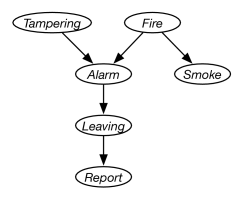
Figure 8.3: Belief network for report of leaving of Example 8.15

This network represents the factorization

	$\displaystyle P(Tam$	$\displaystyle pering,Fire,Alarm,Smoke,Leaving,Report)$
	$\displaystyle\mbox{}=\mbox{}$	$\displaystyle P(Tampering)P(Fire)P(Alarm\mid Tampering,Fire)$
		$\displaystyleP(Smoke\mid Fire)P(Leaving\mid Alarm)*P(Report\mid Leaving).$

Note that the alarm is not a smoke alarm, which would affected by the smoke, and not directly by the fire, but rather is a heat alarm that is directly affected by the fire. This is made explicit in the model in that the $A l a r m$ is independent of $S m o k e$ given $F i r e$ .

We also must define the domain of each variable. Assume that the variables are Boolean; that is, they have domain $\{true,false\}$ . We use the lower-case variant of the variable to represent the true value and use negation for the false value. Thus, for example, $Tampering\,{=}\,true$ is written as $t a m p e r i n g$ , and $Tampering\,{=}\,false$ is written as $\neg tampering$ .

The examples that follow assume the following conditional probabilities:

\displaystyle{P(tampering)=0.02}

\displaystyle{P(fire)=0.01}

\displaystyle{P(alarm\mid fire\wedge tampering)=0.5}

\displaystyle{P(alarm\mid fire\wedge\neg tampering)=0.99}

\displaystyle{P(alarm\mid\neg fire\wedge tampering)=0.85}

\displaystyle{P(alarm\mid\neg fire\wedge\neg tampering)=0.0001}

\displaystyle{P(smoke\mid fire)=0.9}

\displaystyle{P(smoke\mid\neg fire)=0.01}

\displaystyle{P(leaving\mid alarm)=0.88}

\displaystyle{P(leaving\mid\neg alarm)=0.001}

\displaystyle{P(report\mid leaving)=0.75}

\displaystyle{P(report\mid\neg leaving)=0.01}

Before any evidence arrives, the probability is given by the priors. The following probabilities follow from the model (all of the numbers here are to about three decimal places):

	$\displaystyle{P(tampering)=0.02}$
	$\displaystyle{P(fire)=0.01}$
	$\displaystyle{P(report)=0.028}$
	$\displaystyle{P(smoke)=0.0189}$

Observing a report gives the following:

	$\displaystyle{P(tampering\mid report)=0.399}$
	$\displaystyle{P(fire\mid report)=0.2305}$
	$\displaystyle{P(smoke\mid report)=0.215}$

As expected, the probabilities of both $t a m p e r i n g$ and $f i r e$ are increased by the report. Because the probability of $f i r e$ is increased, so is the probability of $s m o k e$ .

Suppose instead that $s m o k e$ alone was observed:

	$\displaystyle{P(tampering\mid smoke)=0.02}$
	$\displaystyle{P(fire\mid smoke)=0.476}$
	$\displaystyle{P(report\mid smoke)=0.320}$

Note that the probability of $t a m p e r i n g$ is not affected by observing $s m o k e$ ; however, the probabilities of $r e p o r t$ and $f i r e$ are increased.

Suppose that both $r e p o r t$ and $s m o k e$ were observed:

	$\displaystyle{P(tampering\mid report\wedge smoke)=0.0284}$
	$\displaystyle{P(fire\mid report\wedge smoke)=0.964}$

Observing both makes $f i r e$ even more likely. However, in the context of the $r e p o r t$ , the presence of $s m o k e$ makes $t a m p e r i n g$ less likely. This is because the $r e p o r t$ is explained away by $f i r e$ , which is now more likely.

Suppose instead that $r e p o r t$ , but not $s m o k e$ , was observed:

	$\displaystyle{P(tampering\mid report\wedge\neg smoke)=0.501}$
	$\displaystyle{P(fire\mid report\wedge\neg smoke)=0.0294}$

In the context of the $r e p o r t$ , $f i r e$ becomes much less likely and so the probability of $t a m p e r i n g$ increases to explain the $r e p o r t$ .

This example illustrates how the belief net independence assumption gives commonsense conclusions and also demonstrates how explaining away is a consequence of the independence assumption of a belief network.

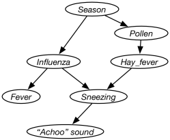
Example 8.16.

Consider the problem of diagnosing why someone is sneezing and perhaps has a fever. Sneezing could be because of influenza or because of hay fever. They are not independent, but are correlated due to the season. Suppose hay fever depends on the season because it depends on the amount of pollen, which in turn depends on the season. The agent does not get to observe sneezing directly, but rather observed just the “Achoo” sound. Suppose fever depends directly on influenza. These dependency considerations lead to the belief network of Figure 8.4.

Figure 8.5: Belief network for the electrical domain of Figure 1.8

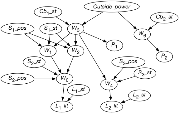
Example 8.17.

Consider the wiring example of Figure 1.8. Suppose we decide to have variables for whether lights are lit, for the switch positions, for whether lights and switches are faulty or not, and for whether there is power in the wires. The variables are defined in Figure 8.5.

We order the variables so that each variable has few parents. In this case there seems to be a natural causal order where, for example, the variable for whether a light is lit comes after variables for whether the light is working and whether there is power coming into the light.

Whether light $l_{1}$ is lit depends only on whether there is power in wire $w_{0}$ and whether light $l_{1}$ is working properly. Other variables, such as the position of switch $s_{1}$ , whether light $l_{2}$ is lit, or who is the Queen of Canada, are irrelevant. Thus, the parents of $L_{1}\_lit$ are $W_{0}$ and $L_{1}\_st$ .

Consider variable $W_{0}$ , which represents whether there is power in wire $w_{0}$ . If we knew whether there was power in wires $w_{1}$ and $w_{2}$ , and we knew the position of switch $s_{2}$ and whether the switch was working properly, the value of the other variables (other than $L_{1}\_lit$ ) would not affect our belief in whether there is power in wire $w_{0}$ . Thus, the parents of $W_{0}$ should be $S_{2}\_Pos$ , $S_{2}\_st$ , $W_{1}$ , and $W_{2}$ .

Figure 8.5 shows the resulting belief network after the independence of each variable has been considered. The belief network also contains the domains of the variables, as given in the figure, and conditional probabilities of each variable given its parents.

For the variable $W_{1}$ , the following conditional probabilities must be specified:

	$\displaystyle{P(W_{1}=live\mid S_{1}\_pos=up\wedge\mbox{}S_{1}\_st=ok\wedge% \mbox{}W_{3}=live)}$
	$\displaystyle{P(W_{1}=live\mid S_{1}\_pos=up\wedge\mbox{}S_{1}\_st=ok\wedge% \mbox{}W_{3}=dead)}$
	$\displaystyle{P(W_{1}=live\mid S_{1}\_pos=up\wedge\mbox{}S_{1}\_st=upside\_% down\wedge\mbox{}W_{3}=live)}$
	$\displaystyle\ \ \ \ {\vdots}$
	$\displaystyle{P(W_{1}=live\mid S_{1}\_pos=down\wedge\mbox{}S_{1}\_st=broken% \wedge\mbox{}W_{3}=dead).}$

There are two values for $S_{1}\_pos$ , five values for $S_{1}\_ok$ , and two values for $W_{3}$ , so there are $2*5*2=20$ different cases where a value for the conditional probability of $W_{1}=live$ must be specified. As far as probability theory is concerned, the probability for $W_{1}=live$ for these 20 cases could be assigned arbitrarily. Of course, knowledge of the domain constrains what values make sense. The values for $W_{1}=dead$ can be computed from the values for $W_{1}=live$ for each of these cases.

Because the variable $S_{1}\_st$ has no parents, it requires a prior distribution, which can be specified as the probabilities for all but one of the values; the remaining value is derived from the constraint that all of the probabilities sum to 1. Thus, to specify the distribution of $S_{1}\_st$ , four of the following five probabilities must be specified:

	$\displaystyle{P(S_{1}\_st=ok)}$
	$\displaystyle{P(S_{1}\_st=upside\_down)}$
	$\displaystyle{P(S_{1}\_st=short)}$
	$\displaystyle{P(S_{1}\_st=intermittent)}$
	$\displaystyle{P(S_{1}\_st=broken)}$

The other variables are represented analogously.

Such a network is used in a number of ways:

•

By conditioning on the knowledge that the switches and circuit breakers are ok, and on the values of the outside power and the position of the switches, this network simulates how the lighting should work.
•

Given values of the outside power and the position of the switches, the network can infer the probability of any outcome, such as how likely it is that $l_{1}$ is lit.
•

Given values for the switches and whether the lights are lit, the posterior probability that each switch or circuit breaker is in any particular state can be inferred.
•

Given some observations, the network may be used to determine the most likely position of switches.
•

Given some switch positions, some outputs, and some intermediate values, the network may be used to determine the probability of any other variable in the network.

Note the independence assumption embedded in this model. The DAG specifies that the lights, switches, and circuit breakers break independently. To model dependencies among how the switches break, you could add more arcs and perhaps more variables. For example, if some lights do not break independently because they come from the same batch, you could add an extra node modeling the batch, and whether it is a good batch or a bad batch, which is made a parent of the $L_{i}\_st$ variables for each light $L_{i}$ from that batch. The lights now break dependently. When you have evidence that one light is broken, the probability that the batch is bad may increase and thus make it more likely that other lights from that batch are broken. If you are not sure whether the lights are indeed from the same batch, you could add variables representing this, too. The important point is that the belief network provides a specification of independence that lets us model dependencies in a natural and direct manner.

The model implies that there is no possibility of shorts in the wires or that the house is wired differently from the diagram. For example, it implies that $w_{0}$ cannot be shorted to $w_{4}$ so that wire $w_{0}$ gets power from wire $w_{4}$ . You could add extra dependencies that let each possible short be modeled. An alternative is to add an extra node that indicates that the model is appropriate. Arcs from this node would lead to each variable representing power in a wire and to each light. When the model is appropriate, you could use the probabilities of Example 8.17. When the model is inappropriate, you could, for example, specify that each wire and light works at random. When there are weird observations that do not fit in with the original model – they are impossible or extremely unlikely given the model – the probability that the model is inappropriate will increase.

Belief Networks and Causality

Belief networks have often been called causal networks and provide representation of causality that takes noise and probabilities into account. Recall that a causal model predicts the result of interventions, where an intervention is an action to change the value of a variable using a mechanism outside of the model (e.g., putting a light switch up, or artificially reducing the amount of pollen).

To build a causal model of a domain given a set of random variables, create the arcs as follows. For each pair of random variables $X$ and $Y$ , make $X$ a parent of $Y$ if intervening on $X$ (perhaps in some context of other variables) causes $Y$ to have a different value (even probabilistically), and the effect of $X$ on $Y$ cannot be accounted for by having other variables $Z$ so that $X$ affects $Z$ and $Z$ affects $Y$ . The belief network of Figure 8.5 is such a causal network. You would expect that a causal model built in this way would obey the independence assumption of the belief network. Thus, all of the conclusions of the belief network would be valid.

You would also expect such a graph to be acyclic; you do not want something eventually causing itself. This assumption is reasonable if you consider that the random variables represent particular events rather than event types. For example, consider a causal chain that “being stressed” causes you to “work inefficiently,” which, in turn, causes you to “be stressed.” To break the apparent cycle, we represent “being stressed” at different stages as different random variables that refer to different times. Being stressed in the past causes you to not work well at the moment which causes you to be stressed in the future. The variables should satisfy the clarity principle and have a well-defined meaning. The variables should not be seen as event types.

The belief network itself has nothing to say about causation, and it can represent non-causal independence, but it seems particularly appropriate for modeling causality. Adding arcs that represent local causality tends to produce a small belief network.

A causal network models interventions in the following way. If someone were to artificially force a variable to have a particular value, the variable’s descendants – but no other variables – would be affected. In Example 8.16, intervening to add or remove pollen would affect hay fever, sneezing and the sound, but not the other variables. This contrasts with observing pollen which provides evidence of the season, and so the probability of all variables would be affected by the observation.

Finally, see how the causality in belief networks relates to the causal and evidential reasoning discussed in Section 5.8. A causal belief network is a way of axiomatizing in a causal direction. Reasoning in belief networks corresponds to abducing to causes and then predicting from these.

Artificial Intelligence 2E

8.3.2 Constructing Belief Networks

Example 8.15.

Example 8.16.

Example 8.17.

Artificial
Intelligence 2E