Third edition of Artificial Intelligence: foundations of computational agents, Cambridge University Press, 2023 is now available (including the full text).
3.5.1 Depth-First Search
The first strategy is depth-first search. In depth-first search, the frontier acts like a last-in first-out stack. The elements are added to the stack one at a time. The one selected and taken off the frontier at any time is the last element that was added.
Notice how the first six nodes expanded are all in a single path. The sixth node has no neighbors. Thus, the next node that is expanded is a child of the lowest ancestor of this node that has unexpanded children.
Implementing the frontier as a stack results in paths being pursued in a depth-first manner - searching one path to its completion before trying an alternative path. This method is said to involve backtracking: The algorithm selects a first alternative at each node, and it backtracks to the next alternative when it has pursued all of the paths from the first selection. Some paths may be infinite when the graph has cycles or infinitely many nodes, in which case a depth-first search may never stop.
This algorithm does not specify the order in which the neighbors are added to the stack that represents the frontier. The efficiency of the algorithm is sensitive to this ordering.
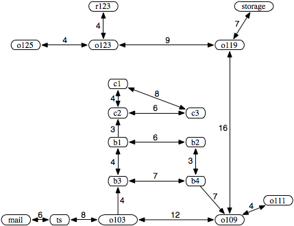
Initially, the frontier contains the trivial path ⟨o103⟩.
At the next stage, the frontier contains the following paths:
[⟨o103,ts⟩,⟨o103,b3⟩,⟨o103,o109⟩].
Next, the path ⟨o103,ts⟩ is selected because it is at the top of the stack. It is removed from the frontier and replaced by extending it by one arc, resulting in the frontier
[⟨o103,ts,mail⟩,⟨o103,b3⟩,⟨o103,o109⟩].
Next, the first path ⟨o103,ts,mail⟩ is removed from the frontier and is replaced by the set of paths that extend it by one arc, which is the empty set because mail has no neighbors. Thus, the resulting frontier is
[⟨o103,b3⟩,⟨o103,o109⟩].
At this stage, the path ⟨o103,b3⟩ is the top of the stack. Notice what has happened: depth-first search has pursued all paths from ts and, when all of these paths were exhausted (there was only one), it backtracked to the next element of the stack. Next, ⟨o103,b3⟩ is selected and is replaced in the frontier by the paths that extend it by one arc, resulting in the frontier
[⟨o103,b3,b1⟩, ⟨o103,b3,b4⟩, ⟨o103,o109⟩].
Then ⟨o103,b3,b1⟩ is selected from the frontier and is replaced by all one-arc extensions, resulting in the frontier
[⟨o103,b3,b1,c2⟩, ⟨o103,b3,b1,b2⟩, ⟨o103,b3,b4⟩, ⟨o103,o109⟩].
Now the first path is selected from the frontier and is extended by one arc, resulting in the frontier
[⟨o103,b3,b1,c2, c3⟩, ⟨o103,b3,b1,c2, c1⟩, ⟨o103,b3,b1,b2⟩, ⟨o103,b3,b4⟩,⟨o103,o109⟩].
Node c3 has no neighbors, and thus the search "backtracks" to the last alternative that has not been pursued, namely to the path to c1.
Suppose ⟨n0,...,nk⟩ is the selected path in the frontier. Then every other element of the frontier is of the form ⟨n0,...,ni,m⟩, for some index i<k and some node m that is a neighbor of ni; that is, it follows the selected path for a number of arcs and then has exactly one extra node.
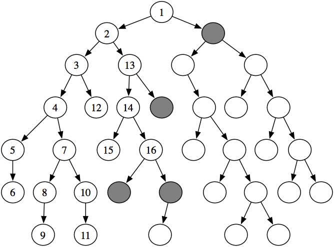
To understand the complexity (see the box) of depth-first search, consider an analogy using family trees, where the neighbors of a node correspond to its children in the tree. At the root of the tree is a start node. A branch down this tree corresponds to a path from a start node. Consider the node at the end of path at the top of the frontier. The other elements of the frontier correspond to children of ancestors of that node - the "uncles," "great uncles," and so on. If the branching factor is b and the first element of the list has length n, there can be at most n×(b-1) other elements of the frontier. These elements correspond to the b-1 alternative paths from each node. Thus, for depth-first search, the space used is linear in the depth of the path length from the start to a node.
Comparing Algorithms
Algorithms (including search algorithms) can be compared on
- the time taken,
- the space used, and
- the quality or accuracy of the results.
The time taken, space used, and accuracy of an algorithm are a function of the inputs to the algorithm. Computer scientists talk about the asymptotic complexity of algorithms, which specifies how the time or space grows with the input size of the algorithm. An algorithm has time (or space) complexity O(f(n)) - read "big-oh of f(n)" - for input size n, where f(n) is some function of n, if there exist constants n0 and k such that the time, or space, of the algorithm is less than k×f(n) for all n>n0. The most common types of functions are exponential functions such as 2n, 3n, or 1.015n; polynomial functions such as n5, n2, n, or n1/2; and logarithmic functions, log n. In general, exponential algorithms get worse more quickly than polynomial algorithms which, in turn, are worse than logarithmic algorithms.
An algorithm has time or space complexity Ω(f(n)) for input size n if there exist constants n0 and k such that the time or space of the algorithm is greater than k×f(n) for all n>n0. An algorithm has time or space complexity Θ(n) if it has complexity O(n) and Ω(n). Typically, you cannot give an Θ(f(n)) complexity on an algorithm, because most algorithms take different times for different inputs. Thus, when comparing algorithms, one has to specify the class of problems that will be considered.
Algorithm A is better than B, using a measure of either time, space, or accuracy, could mean:
- the worst case of A is better than the worst case of B; or
- A works better in practice, or the average case of A is better than the average case of B, where you average over typical problems; or
- you characterize the class of problems for which A is better than B, so that which algorithm is better depends on the problem; or
- for every problem, A is better than B.
The worst-case asymptotic complexity is often the easiest to show, but it is usually the least useful. Characterizing the class of problems for which one algorithm is better than another is usually the most useful, if it is easy to determine which class a given problem is in. Unfortunately, this characterization is usually very difficult.
Characterizing when one algorithm is better than the other can be done either theoretically using mathematics or empirically by building implementations. Theorems are only as valid as the assumptions on which they are based. Similarly, empirical investigations are only as good as the suite of test cases and the actual implementations of the algorithms. It is easy to disprove a conjecture that one algorithm is better than another for some class of problems by showing a counterexample, but it is much more difficult to prove such a conjecture.
If there is a solution on the first branch searched, then the time complexity is linear in the length of the path; it considers only those elements on the path, along with their siblings. The worst-case complexity is infinite. Depth-first search can get trapped on infinite branches and never find a solution, even if one exists, for infinite graphs or for graphs with loops. If the graph is a finite tree, with the forward branching factor bounded by b and depth n, the worst-case complexity is O(bn).
[⟨o103,ts⟩, ⟨o103,b3⟩, ⟨o103,o109⟩]
[⟨o103,ts,mail⟩, ⟨o103,ts,o103⟩, ⟨o103,b3⟩, ⟨o103,o109⟩]
[⟨o103,ts,mail,ts⟩, ⟨o103,ts,o103⟩, ⟨o103,b3⟩, ⟨o103,o109⟩]
[⟨o103,ts,mail,ts,mail⟩, ⟨o103,ts,mail,ts,o103⟩, ⟨o103,ts,o103⟩,
⟨o103,b3⟩, ⟨o103,o109⟩]
Depth-first search can be improved by not considering paths with cycles.
Because depth-first search is sensitive to the order in which the neighbors are added to the frontier, care must be taken to do it sensibly. This ordering can be done statically (so that the order of the neighbors is fixed) or dynamically (where the ordering of the neighbors depends on the goal).
Depth-first search is appropriate when either
- space is restricted;
- many solutions exist, perhaps with long path lengths, particularly for the case where nearly all paths lead to a solution; or
- the order of the neighbors of a node are added to the stack can be tuned so that solutions are found on the first try.
It is a poor method when
- it is possible to get caught in infinite paths; this occurs when the graph is infinite or when there are cycles in the graph; or
- solutions exist at shallow depth, because in this case the search may look at many long paths before finding the short solutions.
Depth-first search is the basis for a number of other algorithms, such as iterative deepening.
