Third edition of Artificial Intelligence: foundations of computational agents, Cambridge University Press, 2023 is now available (including the full text).
3.3.1 Formalizing Graph Searching
A directed graph consists of
In this definition, a node can be anything. All this definition does is constrain arcs to be ordered pairs of nodes. There can be infinitely many nodes and arcs. We do not assume that the graph is represented explicitly; we require only a procedure that can generate nodes and arcs as needed.
The arc ⟨n1,n2⟩ is an outgoing arc from n1 and an incoming arc to n2.
A node n2 is a neighbor of n1 if there is an arc from n1 to n2; that is, if ⟨n1,n2⟩∈A. Note that being a neighbor does not imply symmetry; just because n2 is a neighbor of n1 does not mean that n1 is necessarily a neighbor of n2. Arcs may be labeled, for example, with the action that will take the agent from one state to another.
A path from node s to node g is a sequence of nodes ⟨n0, n1,..., nk⟩ such that s=n0, g=nk, and ⟨ni-1,ni⟩∈A; that is, there is an arc from ni-1 to ni for each i. Sometimes it is useful to view a path as the sequence of arcs, ⟨no,n1⟩, ⟨n1,n2⟩,..., ⟨nk-1,nk⟩ , or a sequence of labels of these arcs.
A cycle is a nonempty path such that the end node is the same as the start node - that is, a cycle is a path ⟨n0, n1,..., nk⟩ such that n0=nk and k≠0. A directed graph without any cycles is called a directed acyclic graph (DAG). This should probably be an acyclic directed graph, because it is a directed graph that happens to be acyclic, not an acyclic graph that happens to be directed, but DAG sounds better than ADG!
A tree is a DAG where there is one node with no incoming arcs and every other node has exactly one incoming arc. The node with no incoming arcs is called the root of the tree and nodes with no outgoing arcs are called leaves.
To encode problems as graphs, one set of nodes is referred to as the start nodes and another set is called the goal nodes. A solution is a path from a start node to a goal node.
Sometimes there is a cost - a positive number - associated with arcs. We write the cost of arc ⟨ni,nj⟩ as cost(⟨ni,nj⟩). The costs of arcs induces a cost of paths.
Given a path p = ⟨n0, n1,..., nk⟩, the cost of path p is the sum of the costs of the arcs in the path:
cost(p) = cost(⟨n0,n1⟩) + ...+ cost(⟨nk-1,nk⟩)
An optimal solution is one of the least-cost solutions; that is, it is a path p from a start node to a goal node such that there is no path p' from a start node to a goal node where cost(p')<cost(p).
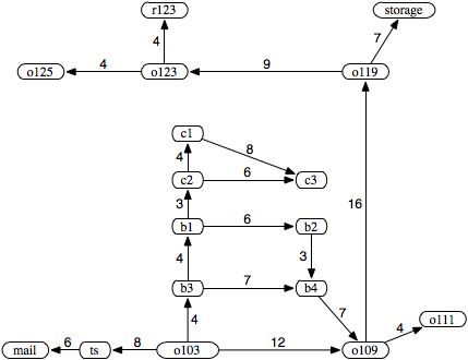
In this graph, the nodes are N={mail,ts,o103,b3,o109,...} and the arcs are A={⟨ts,mail⟩, ⟨o103,ts⟩, ⟨o103,b3⟩, ⟨o103,o109⟩, ...}. Node o125 has no neighbors. Node ts has one neighbor, namely mail. Node o103 has three neighbors, namely ts, b3, and o109.
There are three paths from o103 to r123:
⟨o103, o109, o119, o123, r123⟩ ⟨o103, b3, b4, o109, o119, o123, r123⟩ ⟨o103, b3, b1, b2, b4, o109, o119, o123, r123⟩
If o103 were a start node and r123 were a goal node, each of these three paths would be a solution to the graph-searching problem.
In many problems the search graph is not given explicitly; it is dynamically constructed as needed. All that is required for the search algorithms that follow is a way to generate the neighbors of a node and to determine if a node is a goal node.
The forward branching factor of a node is the number of arcs leaving the node. The backward branching factor of a node is the number of arcs entering the node. These factors provide measures of the complexity of graphs. When we discuss the time and space complexity of the search algorithms, we assume that the branching factors are bounded from above by a constant.
The branching factor is important because it is a key component in the size of the graph. If the forward branching factor for each node is b, and the graph is a tree, there are bn nodes that are n arcs away from any node.
