Third edition of Artificial Intelligence: foundations of computational agents, Cambridge University Press, 2023 is now available (including the full text).
2.3 Hierarchical Control
One way that you could imagine building an agent depicted in Figure 2.1 is to split the body into the sensors and a complex perception system that feeds a description of the world into a reasoning engine implementing a controller that, in turn, outputs commands to actuators. This turns out to be a bad architecture for intelligent systems. It is too slow, and it is difficult to reconcile the slow reasoning about complex, high-level goals with the fast reaction that an agent needs, for example, to avoid obstacles. It also is not clear that there is a description of a world that is independent of what you do with it (see Exercise 2.1).
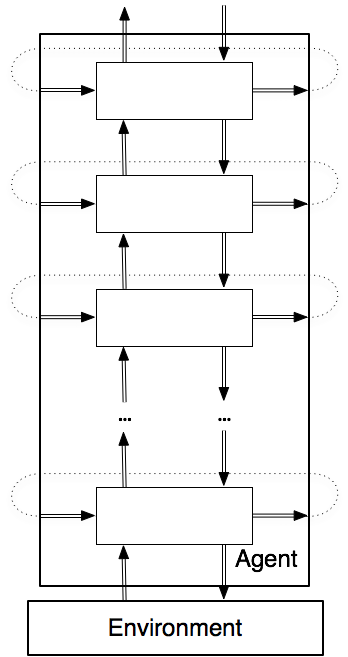
An alternative architecture is a hierarchy of controllers as depicted in Figure 2.4. Each layer sees the layers below it as a virtual body from which it gets percepts and to which it sends commands. The lower-level layers are able to run much faster, react to those aspects of the world that need to be reacted to quickly, and deliver a simpler view of the world to the higher layers, hiding inessential information.
In general, there can be multiple features passed from layer to layer and between states at different times.
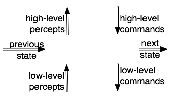
There are three types of inputs to each layer at each time:
- the features that come from the belief state, which are referred to as the remembered or previous values of these features;
- the features representing the percepts from the layer below in the hierarchy; and
- the features representing the commands from the layer above in the hierarchy.
There are three types of outputs from each layer at each time:
- the higher-level percepts for the layer above,
- the lower-level commands for the layer below, and
- the next values for the belief-state features.
An implementation of a layer specifies how the outputs of a layer are a function of its inputs. Computing this function can involve arbitrary computation, but the goal is to keep each layer as simple as possible.
To implement a controller, each input to a layer must get its value from somewhere. Each percept or command input should be connected to an output of some other layer. Other inputs come from the remembered beliefs. The outputs of a layer do not have to be connected to anything, or they could be connected to multiple inputs.
High-level reasoning, as carried out in the higher layers, is often discrete and qualitative, whereas low-level reasoning, as carried out in the lower layers, is often continuous and quantitative (see box). A controller that reasons in terms of both discrete and continuous values is called a hybrid system.
Qualitative Versus Quantitative Representations
Much of science and engineering considers quantitative reasoning with numerical quantities, using differential and integral calculus as the main tools. Qualitative reasoning is reasoning, often using logic, about qualitative distinctions rather than numerical values for given parameters.
Qualitative reasoning is important for a number of reasons:
- An agent may not know what the exact values are. For example, for the delivery robot to pour coffee, it may not be able to compute the optimal angle that the coffee pot needs to be tilted, but a simple control rule may suffice to fill the cup to a suitable level.
- The reasoning may be applicable regardless of the quantitative values. For example, you may want a strategy for a robot that works regardless of what loads are placed on the robot, how slippery the floors are, or what the actual charge is of the batteries, as long as they are within some normal operating ranges.
- An agent needs to do qualitative reasoning to determine which quantitative laws are applicable. For example, if the delivery robot is filling a coffee cup, different quantitative formulas are appropriate to determine where the coffee goes when the coffee pot is not tilted enough for coffee to come out, when coffee comes out into a non-full cup, and when the coffee cup is full and the coffee is soaking into the carpet.
Qualitative reasoning uses discrete values, which can take a number of forms:
- Landmarks are values that make qualitative distinctions in the individual being modeled. In the coffee example, some important qualitative distinctions include whether the coffee cup is empty, partially full, or full. These landmark values are all that is needed to predict what happens if the cup is tipped upside down or if coffee is poured into the cup.
- Orders-of-magnitude reasoning involves approximate reasoning that ignores minor distinctions. For example, a partially full coffee cup may be full enough to deliver, half empty, or nearly empty. These fuzzy terms have ill-defined borders. Some relationship exists between the actual amount of coffee in the cup and the qualitative description, but there may not be strict numerical divisors.
- Qualitative derivatives indicate whether some value is increasing, decreasing, or staying the same.
A flexible agent needs to do qualitative reasoning before it does quantitative reasoning. Sometimes qualitative reasoning is all that is needed. Thus, an agent does not always need to do quantitative reasoning, but sometimes it needs to do both qualitative and quantitative reasoning.
Assume the delivery robot has wheels like a car, and at each time can either go straight, turn right, or turn left. It cannot stop. The velocity is constant and the only command is to set the steering angle. Turning the wheels is instantaneous, but adjusting to a certain direction takes time. Thus, the robot can only travel straight ahead or go around in circular arcs with a fixed radius.
The robot has a position sensor that gives its current coordinates and orientation. It has a single whisker sensor that sticks out in front and slightly to the right and detects when it has hit an obstacle. In the example below, the whisker points 30o to the right of the direction the robot is facing. The robot does not have a map, and the environment can change (e.g., obstacles can move).
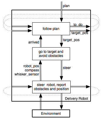
A layered controller for such a delivery robot is depicted in Figure 2.5. The robot is given a high-level plan to execute. The plan is a sequence of named locations to visit in order. The robot needs to sense the world and to move in the world in order to carry out the plan. The details of the lower layer are not shown in this figure.
The top layer, called follow plan, is described in Example 2.6. That layer takes in a plan to execute. The plan is a list of named locations to visit in order. The locations are selected in order. Each selected location becomes the current target. This layer determines the x-y coordinates of the target. These coordinates are the target position for the lower level. The upper level knows about the names of locations, but the lower levels only know about coordinates.
The top layer maintains a belief state consisting of a list of names of locations that the robot still needs to visit and the coordinates of the current target. It issues commands to the middle layer in terms of the coordinates of the current target.
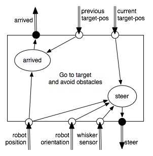
The middle layer, which could be called go to target and avoid obstacles, tries to keep traveling toward the current target position, avoiding obstacles. The middle layer is described in Example 2.5. The target position, target_pos, is obtained from the top layer. When the middle layer has arrived at the target position, it signals to the top layer that it has achieved the target by setting arrived to be true. This signal can be implemented either as the middle layer issuing an interrupt to the top layer, which was waiting, or as the top layer continually monitoring the middle layer to determine when arrived becomes true. When arrived becomes true, the top layer then changes the target position to the coordinates of the next location on the plan. Because the top layer changes the current target position, the middle layer must use the previous target position to determine whether it has arrived. Thus, the middle layer must get both the current and the previous target positions from the top layer: the previous target position to determine whether it has arrived, and the current target position to travel to.
The middle layer can access the robot's current position and direction and can determine whether its single whisker sensor is on or off. It can use a simple strategy of trying to head toward the target unless it is blocked, in which case it turns left.
The middle layer is built on a lower layer that provides a simple view of the robot. This lower layer could be called steer robot and report obstacles and position. It takes in steering commands and reports the robot's position, orientation, and whether the sensor is on or off.
Inside a layer are features that can be functions of other features and of the inputs to the layers. There is an arc into a feature from the features or inputs on which it is dependent. The graph of how features depend on each other must be acyclic. The acyclicity of the graph allows the controller to be implemented by running a program that assigns the values in order. The features that make up the belief state can be written to and read from memory.
The robot has a single whisker sensor that detects obstacles touching the whisker. The one bit value that specifies whether the whisker sensor has hit an obstacle is provided by the lower layer. The lower layer also provides the robot position and orientation. All the robot can do is steer left by a fixed angle, steer right, or go straight. The aim of this layer is to make the robot head toward its current target position, avoiding obstacles in the process, and to report when it has arrived.
This layer of the controller maintains no internal belief state, so the belief state transition function is vacuous. The command function specifies the robot's steering direction as a function of its inputs and whether the robot has arrived.
The robot has arrived if its current position is close to the previous target position. Thus, arrived is assigned a value that is a function of the robot position and previous target position, and a threshold constant:
arrived ←distance(previous_target_pos,robot_pos)<threshold
where ← means assignment, distance is the Euclidean distance, and threshold is a distance in the appropriate units.
The robot steers left if the whisker sensor is on; otherwise it heads toward the target position. This can be achieved by assigning the appropriate value to the steer variable:
then steer←left
else if straight_ahead(robot_pos,robot_dir,current_target_pos)
then steer←straight
else if left_of(robot_position,robot_dir,current_target_pos)
then steer←left
else steer←right
end if
where straight_ahead(robot_pos,robot_dir,current_target_pos) is true when the robot is at robot_pos, facing the direction robot_dir, and when the current target position, current_target_pos, is straight ahead of the robot with some threshold (for later examples, this threshold is 11o of straight ahead). The function left_of tests if the target is to the left of the robot.
This layer is purely quantitative. It reasons in terms of numerical quantities rather than discrete values.
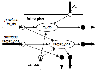
This layer maintains an internal belief state. It remembers the current target position and what locations it still has to visit. The to_do feature has as its value a list of all pending locations to visit. The target_pos feature maintains the position for the current target.
Once the robot has arrived at its previous target, the next target position is the coordinate of the next location to visit. The top-level plan given to the robot is in terms of named locations, so these must be translated into coordinates for the middle layer to use. The following code shows how the target position and the to_do list are changed when the robot has arrived at its previous target position:
then
target_pos' ←coordinates(head(to_do))
to_do'←tail(to_do)
end if
where to_do' is the next value for the to_do feature, and target_pos' is the next target position. Here head(to_do) is the first element of the to_do list, tail(to_do) is the rest of the to_do list, and empty(to_do) is true when the to_do list is empty.
In this layer, if the to_do list becomes empty, the robot does not change its target position. It keeps going around in circles. See Exercise 2.3.
This layer determines the coordinates of the named locations. This could be done by simply having a database that specifies the coordinates of the locations. Using such a database is sensible if the locations do not move and are known a priori. However, if the locations can move, the lower layer must be able to tell the upper layer the current position of a location. The top layer would have to ask the lower layer the coordinates of a given location. See Exercise 2.8.
To complete the controller, the belief state variables must be initialized, and the top-level plan must be input. This can be done by initializing the to_do list with the tail of the plan and the target_pos with the location of the first location. A simulation of the plan [goto(o109),goto(storage),goto(o109),goto(o103)] with one obstacle is given in Figure 2.8. The robot starts at position (0,5) facing 90o (north), and there is a rectangular obstacle between the positions (20,20) and (35,-5).