Third edition of Artificial Intelligence: foundations of computational agents, Cambridge University Press, 2023 is now available (including the full text).
7.8 Bayesian Learning
Rather than choosing the most likely model or delineating the set of all models that are consistent with the training data, another approach is to compute the posterior probability of each model given the training examples.
The idea of Bayesian learning is to compute the posterior probability distribution of the target features of a new example conditioned on its input features and all of the training examples.
Suppose a new case has inputs X=x and has target features, Y; the aim is to compute P(Y|X=x∧e), where e is the set of training examples. This is the probability distribution of the target variables given the particular inputs and the examples. The role of a model is to be the assumed generator of the examples. If we let M be a set of disjoint and covering models, then reasoning by cases and the chain rule give
P(Y|x∧e) = ∑m∈M P(Y ∧m |x∧e) = ∑m∈M P(Y | m ∧x∧e) ×P(m|x∧e) = ∑m∈M P(Y | m ∧x) ×P(m|e) .
The first two equalities are theorems from the definition of probability. The last equality makes two assumptions: the model includes all of the information about the examples that is necessary for a particular prediction [i.e., P(Y | m ∧x∧e)= P(Y | m ∧x) ], and the model does not change depending on the inputs of the new example [i.e., P(m|x∧e)= P(m|e)]. This formula says that we average over the prediction of all of the models, where each model is weighted by its posterior probability given the examples.
P(m|e) can be computed using Bayes' rule:
P(m|e) = (P(e|m)×P(m))/(P(e)) .
Thus, the weight of each model depends on how well it predicts the data (the likelihood) and its prior probability. The denominator, P(e), is a normalizing constant to make sure the posterior probabilities of the models sum to 1. Computing P(e) can be very difficult when there are many models.
A set {e1,...,ek} of examples are i.i.d. (independent and identically distributed), where the distribution is given by model m if, for all i and j, examples ei and ej are independent given m, which means P(ei∧ej|m)=P(ei|m)×P(ej|m). We usually assume that the examples are i.i.d.
Suppose the set of training examples e is {e1,...,ek}. That is, e is the conjunction of the ei, because all of the examples have been observed to be true. The assumption that the examples are i.i.d. implies
P(e|m) = ∏i=1k P(ei|m) .
The set of models may include structurally different models in addition to models that differ in the values of the parameters. One of the techniques of Bayesian learning is to make the parameters of the model explicit and to determine the distribution over the parameters.
There is a single parameter, φ, that determines the set of all models. Suppose that φ represents the probability of Y=true. We treat this parameter as a real-valued random variable on the interval [0,1]. Thus, by definition of φ, P(a|φ)=φ and P(¬a|φ)=1-φ.
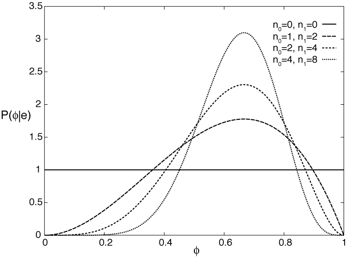
Suppose an agent has no prior information about the probability of Boolean variable Y and no knowledge beyond the training examples. This ignorance can be modeled by having the prior probability distribution of the variable φ as a uniform distribution over the interval [0,1]. This is the the probability density function labeled n0=0, n1=0 in Figure 7.15.
We can update the probability distribution of φ given some examples. Assume that the examples, obtained by running a number of independent experiments, are a particular sequence of outcomes that consists of n0 cases where Y is false and n1 cases where Y is true.
The posterior distribution for φ given the training examples can be derived by Bayes' rule. Let the examples e be the particular sequence of observation that resulted in n1 occurrences of Y=true and n0 occurrences of Y=false. Bayes' rule gives us
P(φ|e)=(P(e|φ)×P(φ))/(P(e)) .
The denominator is a normalizing constant to make sure the area under the curve is 1.
Given that the examples are i.i.d.,
P(e|φ)=φn1×(1-φ)n0
because there are n0 cases where Y=false, each with a probability of 1-φ, and n1 cases where Y=true, each with a probability of φ.
One possible prior probability, P(φ), is a uniform distribution on the interval [0,1]. This would be reasonable when the agent has no prior information about the probability.
Figure 7.15 gives some posterior distributions of the variable φ based on different sample sizes, and given a uniform prior. The cases are (n0=1, n1=2), (n0=2, n1=4), and (n0=4, n1=8). Each of these peak at the same place, namely at (2)/(3). More training examples make the curve sharper.
The distribution of this example is known as the beta distribution; it is parametrized by two counts, α0 and α1, and a probability p. Traditionally, the αi parameters for the beta distribution are one more than the counts; thus, αi=ni+1. The beta distribution is
Betaα0,α1(p)=(1)/(K) pα1-1×(1-p)α0-1
where K is a normalizing constant that ensures the integral over all values is 1. Thus, the uniform distribution on [0,1] is the beta distribution Beta1,1.
The generalization of the beta distribution to more than two parameters is known as the Dirichlet distribution. The Dirichlet distribution with two sorts of parameters, the "counts" α1,...,αk, and the probability parameters p1,...,pk, is
Dirichletα1,...,αk(p1,...,pk) = (1)/(K) ∏j=1k pjαj-1
where K is a normalizing constant that ensures the integral over all values is 1; pi is the probability of the ith outcome (and so 0 ≤ pi ≤ 1) and αi is one more than the count of the ith outcome. That is, αi=ni+1. The Dirichlet distribution looks like Figure 7.15 along each dimension (i.e., as each pj varies between 0 and 1).
For many cases, summing over all models weighted by their posterior distribution is difficult, because the models may be complicated (e.g., if they are decision trees or even belief networks). However, for the Dirichlet distribution, the expected value for outcome i (averaging over all pj's) is
(αi)/(∑j αj) .
The reason that the αi parameters are one more than the counts is to make this formula simple. This fraction is well defined only when the αj are all non-negative and not all are zero.
Thus, the expected value of the n0=1, n1=2 curve is (3)/(5), for the n0=2, n1=4 case the expected value is (5)/(8), and for the n0=4, n1=8 case it is (9)/(14). As the learner gets more training examples, this value approaches (n)/(m).
This estimate is better than (n)/(m) for a number of reasons. First, it tells us what to do if the learning agent has no examples: Use the uniform prior of (1)/(2). This is the expected value of the n=0, m=0 case. Second, consider the case where n=0 and m=3. The agent should not use P(y)=0, because this says that Y is impossible, and it certainly does not have evidence for this! The expected value of this curve with a uniform prior is (1)/(5).
An agent does not have to start with a uniform prior; it can start with any prior distribution. If the agent starts with a prior that is a Dirichlet distribution, its posterior will be a Dirichlet distribution. The posterior distribution can be obtained by adding the observed counts to the αi parameters of the prior distribution.
The i.i.d. assumption can be represented as a belief network, where each of the ei are independent given model m. This independence assumption can be represented by the belief network shown on the left side of Figure 7.16.
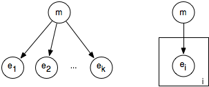
If m is made into a discrete variable, any of the inference methods of the previous chapter can be used for inference in this network. A standard reasoning technique in such a network is to condition on all of the observed ei and to query the model variable or an unobserved ei variable.
The problem with specifying a belief network for a learning problem is that the model grows with the number of observations. Such a network can be specified before any observations have been received by using a plate model. A plate model specifies what variables will be used in the model and what will be repeated in the observations. The right side of Figure 7.16 shows a plate model that represents the same information as the left side. The plate is drawn as a rectangle that contains some nodes, and an index (drawn on the bottom right of the plate). The nodes in the plate are indexed by the index. In the plate model, there are multiple copies of the variables in the plate, one for each value of the index. The intuition is that there is a pile of plates, one for each value of the index. The number of plates can be varied depending on the number of observations and what is queried. In this figure, all of the nodes in the plate share a common parent. The probability of each copy of a variable in a plate given the parents is the same for each index.
A plate model lets us specify more complex relationships between the variables. In a hierarchical Bayesian model, the parameters of the model can depend on other parameters. Such a model is hierarchical in the sense that some parameters can depend on other parameters.
Suppose that for patient X in hospital H there is a random variable SHX that is true when the patient is sick with the flu. (Assume that the patient identification number and the hospital uniquely determine the patient.) There is a value φH for each hospital H that will be used for the prior probability of being sick with the flu for each patient in H. In a Bayesian model, φH is treated as a real-valued random variable with domain [0,1]. SHX depends on φH, with P(SHX|φH)=φH. Assume that φH is distributed according to a beta distribution. We don't assume that φhi and φh2 are independent of each other, but depend on hyperparameters. The hyperparameters can be the prior counts α0 and α1. The parameters depend on the hyperparameters in terms of the conditional probability P(φhi|α0,α1)= Betaα0,α1(φhi); α0 and α1 are real-valued random variables, which require some prior distribution.
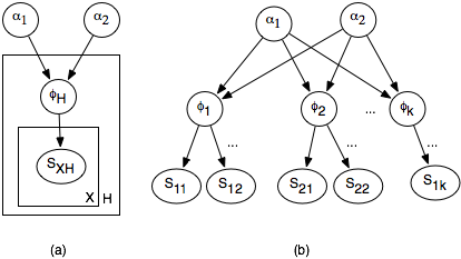
The plate model and the corresponding belief network are shown in Figure 7.17. Part (a) shows the plate model, where there is a copy of the outside plate for each hospital and a copy of the inside plate for each patient in the hospital. Part of the resulting belief network is shown in part (b). Observing some of the SHX will affect the φH and so α0 and α1, which will in turn affect the other φH variables and the unobserved SHX variables.
Sophisticated methods exist to evaluate such networks. However, if the variables are made discrete, any of the methods of the previous chapter can be used.
In addition to using the posterior distribution of φ to derive the expected value, we can use it to answer other questions such as: What is the probability that the posterior probability of φ is in the range [a,b]? In other words, derive P((φ ≥ a ∧φ ≤ b) | e). This is the problem that the Reverend Thomas Bayes solved more than 200 years ago [Bayes(1763)]. The solution he gave - although in much more cumbersome notation - was
(∫ab pn×(1-p)m-n)/(∫01 pn×(1-p)m-n) .
This kind of knowledge is used in surveys when it may be reported that a survey is correct with an error of at most 5%, 19 times out of 20. It is also the same type of information that is used by probably approximately correct (PAC) learning, which guarantees an error at most ε at least 1-δ of the time. If an agent chooses the midpoint of the range [a,b], namely (a+b)/(2), as its hypothesis, it will have error less than or equal to (b-a)/(2), just when the hypothesis is in [a,b]. The value 1-δ corresponds to P(φ ≥ a ∧φ ≤ b | e). If ε=(b-a)/(2) and δ=1-P(φ ≥ a ∧φ ≤ b | e), choosing the midpoint will result in an error at most ε in 1-δ of the time. PAC learning gives worst-case results, whereas Bayesian learning gives the expected number. Typically, the Bayesian estimate is more accurate, but the PAC results give a guarantee of the error. The sample complexity (see Section 7.7.2) required for Bayesian learning is typically much less than that of PAC learning - many fewer examples are required to expect to achieve the desired accuracy than are needed to guarantee the desired accuracy.
