Third edition of Artificial Intelligence: foundations of computational agents, Cambridge University Press, 2023 is now available (including the full text).
6.3 Belief Networks
The notion of conditional independence can be used to give a concise representation of many domains. The idea is that, given a random variable X, a small set of variables may exist that directly affect the variable's value in the sense that X is conditionally independent of other variables given values for the directly affecting variables. The set of locally affecting variables is called the Markov blanket. This locality is what is exploited in a belief network. A belief network is a directed model of conditional dependence among a set of random variables. The precise statement of conditional independence in a belief network takes into account the directionality.
To define a belief network, start with a set of random variables that represent all of the features of the model. Suppose these variables are {X1,...,Xn}. Next, select a total ordering of the variables, X1,...,Xn.
The chain rule (Proposition 6.3) shows how to decompose a conjunction into conditional probabilities:
P(X1=v1∧X2=v2∧···∧Xn=vn) = ∏i=1n P(Xi=vi|X1=v1∧···∧Xi-1=vi-1).
Or, in terms of random variables and probability distributions,
P(X1, X2,···, Xn) = ∏i=1n P(Xi|X1, ···, Xi-1).
Define the parents of random variable Xi, written parents(Xi), to be a minimal set of predecessors of Xi in the total ordering such that the other predecessors of Xi are conditionally independent of Xi given parents(Xi). That is, parents(Xi) ⊆{X1,...,Xi-1} such that
P(Xi|Xi-1...X1) = P(Xi|parents(Xi)).
If more than one minimal set exists, any minimal set can be chosen to be the parents. There can be more than one minimal set only when some of the predecessors are deterministic functions of others.
We can put the chain rule and the definition of parents together, giving
P(X1, X2,···, Xn) = ∏i=1n P(Xi|parents(Xi)).
The probability over all of the variables, P(X1, X2,···, Xn), is called the joint probability distribution. A belief network defines a factorization of the joint probability distribution, where the conditional probabilities form factors that are multiplied together.
A belief network, also called a Bayesian network, is an acyclic directed graph (DAG), where the nodes are random variables. There is an arc from each element of parents(Xi) into Xi. Associated with the belief network is a set of conditional probability distributions - the conditional probability of each variable given its parents (which includes the prior probabilities of those variables with no parents).
Thus, a belief network consists of
- a DAG, where each node is labeled by a random variable;
- a domain for each random variable; and
- a set of conditional probability distributions giving P(X|parents(X)) for each variable X.
A belief network is acyclic by construction. The way the chain rule decomposes the conjunction gives the ordering. A variable can have only predecessors as parents. Different decompositions can result in different belief networks.
Suppose we use the following variables, all of which are Boolean, in the following order:
- Tampering is true when there is tampering with the alarm.
- Fire is true when there is a fire.
- Alarm is true when the alarm sounds.
- Smoke is true when there is smoke.
- Leaving is true if there are many people leaving the building at once.
- Report is true if there is a report given by someone of people leaving. Report is false if there is no report of leaving.
The variable Report denotes the sensor report that people are leaving. This information is unreliable because the person issuing such a report could be playing a practical joke, or no one who could have given such a report may have been paying attention. This variable is introduced to allow conditioning on unreliable sensor data. The agent knows what the sensor reports, but it only has unreliable evidence about people leaving the building. As part of the domain, assume the following conditional independencies:
- Fire is conditionally independent of Tampering (given no other information).
- Alarm depends on both Fire and Tampering. That is, we are making no independence assumptions about how Alarm depends on its predecessors given this variable ordering.
- Smoke depends only on Fire and is conditionally independent of Tampering and Alarm given whether there is a Fire.
- Leaving only depends on Alarm and not directly on Fire or Tampering or Smoke. That is, Leaving is conditionally independent of the other variables given Alarm.
- Report only directly depends on Leaving.
The belief network of Figure 6.1 expresses these dependencies.
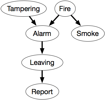
This network represents the factorization
P(Tampering,Fire,Alarm,Smoke,Leaving,Report) = P(Tampering) ×P(Fire) ×P(Alarm|Tampering,Fire) ×P(Smoke|Fire) ×P(Leaving|Alarm) ×P(Report|Leaving).
We also must define the domain of each variable. Assume that the variables are Boolean; that is, they have domain {true,false}. We use the lower-case variant of the variable to represent the true value and use negation for the false value. Thus, for example, Tampering=true is written as tampering, and Tampering=false is written as ¬tampering.
The examples that follow assume the following conditional probabilities:
P(fire) = 0.01
P(alarm | fire ∧tampering) = 0.5
P(alarm | fire ∧¬tampering) = 0.99
P(alarm | ¬fire ∧tampering) = 0.85
P(alarm | ¬fire ∧¬tampering) = 0.0001
P(smoke | fire ) = 0.9
P(smoke | ¬fire ) = 0.01
P(leaving | alarm) = 0.88
P(leaving | ¬alarm ) = 0.001
P(report | leaving ) = 0.75
P(report | ¬leaving ) = 0.01
- For each wire wi, there is a random variable, Wi, with domain {live,dead}, which denotes whether there is power in wire wi. Wi=live means wire wi has power. Wi=dead means there is no power in wire wi.
- Outside_power with domain {live,dead} denotes whether there is power coming into the building.
- For each switch si, variable Si_pos denotes the position of si. It has domain {up,down}.
- For each switch si, variable Si_st denotes the state of switch si. It has domain {ok,upside_down,short,intermittent,broken}. Si_st=ok means switch si is working normally. Si_st=upside_down means switch si is installed upside-down. Si_st=short means switch si is shorted and acting as a wire. Si_st=broken means switch si is broken and does not allow electricity to flow.
- For each circuit breaker cbi, variable Cbi_st has domain {on,off}. Cbi_st=on means power can flow through cbi and Cbi_st=off means that power cannot flow through cbi.
- For each light li, variable Li_st with domain {ok,intermittent,broken} denotes the state of the light. Li_st=ok means light li will light if powered, Li_st=intermittent means light li intermittently lights if powered, and Li_st=broken means light li does not work.
Let's select an ordering where the causes of a variable are before the variable in the ordering. For example, the variable for whether a light is lit comes after variables for whether the light is working and whether there is power coming into the light.
Whether light l1 is lit depends only on whether there is power in wire w0 and whether light l1 is working properly. Other variables, such as the position of switch s1, whether light l2 is lit, or who is the Queen of Canada, are irrelevant. Thus, the parents of L1_lit are W0 and L1_st.
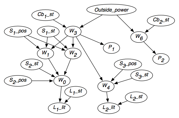
Consider variable W0, which represents whether there is power in wire w0. If we knew whether there was power in wires w1 and w2, and we knew the position of switch s2 and whether the switch was working properly, the value of the other variables (other than L1_lit) would not affect our belief in whether there is power in wire w0. Thus, the parents of W0 should be S2_Pos, S2_st, W1, and W2.
Figure 6.2 shows the resulting belief network after the independence of each variable has been considered. The belief network also contains the domains of the variables, as given in the figure, and conditional probabilities of each variable given its parents.
For the variable W1, the following conditional probabilities must be specified:
P(W1=live|S1_pos=up ∧S1_st=ok ∧W3=live) P(W1=live|S1_pos=up ∧S1_st=ok ∧W3=dead) P(W1=live|S1_pos=up ∧S1_st=upside_down ∧W3=live) ... P(W1=live|S1_pos=down ∧S1_st=broken ∧W3=dead).
There are two values for S1_pos, five values for S1_ok, and two values for W3, so there are 2×5 ×2 = 20 different cases where a value for W1=live must be specified. As far as probability theory is concerned, the probability for W1=live for these 20 cases could be assigned arbitrarily. Of course, knowledge of the domain constrains what values make sense. The values for W1=dead can be computed from the values for W1=live for each of these cases.
Because the variable S1_st has no parents, it requires a prior distribution, which can be specified as the probabilities for all but one of the values; the remaining value can be derived from the constraint that all of the probabilities sum to 1. Thus, to specify the distribution of S1_st, four of the following five probabilities must be specified:
P(S1_st=ok) P(S1_st=upside_down) P(S1_st=short) P(S1_st=intermittent) P(S1_st=broken)
The other variables are represented analogously.
A belief network is a graphical representation of conditional independence. The independence allows us to depict direct effects within the graph and prescribes which probabilities must be specified. Arbitrary posterior probabilities can be derived from the network.
The independence assumption embedded in a belief network is as follows: Each random variable is conditionally independent of its non-descendants given its parents. That is, if X is a random variable with parents Y1,..., Yn, all random variables that are not descendants of X are conditionally independent of X given Y1 ,..., Yn:
P(X|Y1,..., Yn,R)=P(X|Y1,..., Yn),
if R does not involve a descendant of X. For this definition, we include X as a descendant of itself. The right-hand side of this equation is the form of the probabilities that are specified as part of the belief network. R may involve ancestors of X and other nodes as long as they are not descendants of X. The independence assumption states that all of the influence of non-descendant variables is captured by knowing the value of X's parents.
Often, we refer to just the labeled DAG as a belief network. When this is done, it is important to remember that a domain for each variable and a set of conditional probability distributions are also part of the network.
The number of probabilities that must be specified for each variable is exponential in the number of parents of the variable. The independence assumption is useful insofar as the number of variables that directly affect another variable is small. You should order the variables so that nodes have as few parents as possible.
Belief Networks and Causality
Belief networks have often been called causal networks and have been claimed to be a good representation of causality. Recall that a causal model predicts the result of interventions. Suppose you have in mind a causal model of a domain, where the domain is specified in terms of a set of random variables. For each pair of random variables X1 and X2, if a direct causal connection exists from X1 to X2 (i.e., intervening to change X1 in some context of other variables affects X2 and this cannot be modeled by having some intervening variable), add an arc from X1 to X2. You would expect that the causal model would obey the independence assumption of the belief network. Thus, all of the conclusions of the belief network would be valid.
You would also expect such a graph to be acyclic; you do not want something eventually causing itself. This assumption is reasonable if you consider that the random variables represent particular events rather than event types. For example, consider a causal chain that "being stressed" causes you to "work inefficiently," which, in turn, causes you to "be stressed." To break the apparent cycle, we can represent "being stressed" at different stages as different random variables that refer to different times. Being stressed in the past causes you to not work well at the moment which causes you to be stressed in the future. The variables should satisfy the clarity principle and have a well-defined meaning. The variables should not be seen as event types.
The belief network itself has nothing to say about causation, and it can represent non-causal independence, but it seems particularly appropriate when there is causality in a domain. Adding arcs that represent local causality tends to produce a small belief network. The belief network of Figure 6.2 shows how this can be done for a simple domain.
A causal network models interventions. If someone were to artificially force a variable to have a particular value, the variable's descendants - but no other nodes - would be affected. Finally, you can see how the causality in belief networks relates to the causal and evidential reasoning discussed in Section 5.7. A causal belief network can be seen as a way of axiomatizing in a causal direction. Reasoning in belief networks corresponds to abducing to causes and then predicting from these. A direct mapping exists between the logic-based abductive view discussed in Section 5.7 and belief networks: Belief networks can be modeled as logic programs with probabilities over possible hypotheses. This is described in Section 14.3.
Note the restriction "each random variable is conditionally independent of its non-descendants given its parents" in the definition of the independence encoded in a belief network. If R contains a descendant of variable X, the independence assumption is not directly applicable.
The variable S1_pos has no parents. Thus, the independence embedded in the belief network specifies that P(S1_pos=up|A) = P(S1_pos=up) for any A that does not involve a descendant of S1_pos. If A includes a descendant of S1_pos=up - for example, if A is S2_pos=up∧L1_lit=true - the independence assumption cannot be directly applied.
This network can be used in a number of ways:
- By conditioning on the knowledge that the switches and circuit breakers are ok, and on the values of the outside power and the position of the switches, this network can simulate how the lighting should work.
- Given values of the outside power and the position of the switches, the network can infer the likelihood of any outcome - for example, how likely it is that l1 is lit.
- Given values for the switches and whether the lights are lit, the posterior probability that each switch or circuit breaker is in any particular state can be inferred.
- Given some observations, the network can be used to reason backward to determine the most likely position of switches.
- Given some switch positions, some outputs, and some intermediate values, the network can be used to determine the probability of any other variable in the network.
A belief network specifies a joint probability distribution from which arbitrary conditional probabilities can be derived. A network can be queried by asking for the conditional probability of any variables conditioned on the values of any other variables. This is typically done by providing observations on some variables and querying another variable.
P(fire) = 0.01
P(report ) = 0.028
P(smoke) = 0.0189
Observing the report gives the following:
P(fire |report)= 0.2305
P(smoke |report) = 0.215
As expected, the probability of both tampering and fire are increased by the report. Because fire is increased, so is the probability of smoke.
Suppose instead that smoke were observed:
P(fire|smoke) = 0.476
P(report |smoke) = 0.320
Note that the probability of tampering is not affected by observing smoke; however, the probabilities of report and fire are increased.
Suppose that both report and smoke were observed:
P(fire |report ∧smoke) = 0.964
Observing both makes fire even more likely. However, in the context of the report, the presence of smoke makes tampering less likely. This is because the report is explained away by fire, which is now more likely.
Suppose instead that report, but not smoke, was observed:
P(fire|report ∧¬smoke) = 0.0294
In the context of the report, fire becomes much less likely and so the probability of tampering increases to explain the report.
This example illustrates how the belief net independence assumption gives commonsense conclusions and also demonstrates how explaining away is a consequence of the independence assumption of a belief network.
