3 Searching for Solutions 3.7 Pruning the Search Space 3.9 Social Impact

3.8 Search Refinements

A number of refinements can be made to the preceding strategies. The direction of search – searching from the start to a goal or from a goal to the start – can make a difference in efficiency. Backward search can be used to find policies that give an optimal path from any position, and can be used to improve a heuristic function.

3.8.1 Direction of Search

The size of the search space of the generic search algorithm, for a given pruning strategy, depends on the path length and the branching factor. Anything that can be done to reduce these can potentially give great savings. Sometimes it is possible to search backwards from a goal, which can be useful, particularly when it reduces the branching factor.

If the following conditions hold:

•

the set of goal nodes, $\{n:{goal}(n)\}$ , is finite and can be generated
•

for any node $n$ the neighbors of $n$ in the inverse graph, namely $\{n^{\prime}:\left<n^{\prime},n\right>\in A\}$ , can be generated

then the graph-search algorithm can either begin with the start node and search forward for a goal node, or begin with a goal node and search backward for the start node. In many applications, the set of goal nodes, or the inverse graph, cannot easily be generated so backwards search may not be feasible; sometimes the purpose of the search is to just find a goal node and not the path to it.

In backward search, what was the start becomes the goal, and what was the goal becomes the start. If there is a single goal node, it can be used as the start node for backward search. If there can be multiple goal nodes, a new node, ${goal}$ , is created, which becomes the start node of the backward search. The neighbors of ${goal}$ in the backward graph are nodes $\{n:{goal}(n)\}$ . The neighbors of the nodes, apart from $g o a l$ , are given in the inverse graph. The goal of the backward search is the start node of the forward search.

Forward search searches from the start node to the goal nodes in the original graph.

For those cases where the goal nodes and the inverse graph can be generated, it may be more efficient to search in one direction than in the other. The size of the search space is typically exponential in the branching factor. It is often the case that forward and backward searches have different branching factors. A general principle is to search in the direction that has the smaller branching factor.

Bidirectional Search

The idea of bidirectional search is to search forwards from the start and backwards from the goal simultaneously. When the two search frontiers intersect, the algorithm needs to construct a single path that extends from the start node through the frontier intersection to a goal node. It is a challenge to guarantee that the path found is optimal.

A new problem arises during a bidirectional search, namely ensuring that the two search frontiers actually meet. For example, a depth-first search in both directions is not likely to work at all unless one is extremely lucky because its small search frontiers are likely to pass each other by. Breadth-first search in both directions would be guaranteed to meet.

A combination of depth-first search in one direction and breadth-first search in the other would guarantee the required intersection of the search frontiers, but the choice of which to apply in which direction may be difficult. The decision depends on the cost of saving the breadth-first frontier and searching it to check when the depth-first method will intersect one of its elements.

There are situations where a bidirectional search results in substantial savings. For example, if the forward and backward branching factors of the search space are both $b$ , and the goal is at depth $k$ , then breadth-first search will take time proportional to $b^{k}$ , whereas a symmetric bidirectional search will take time proportional to $2b^{k/2}$ , assuming the time overhead of determining intersection is negligible. This is an exponential saving in time, even though the time complexity is still exponential.

Island-Driven Search

One of the ways that search may be made more efficient is to identify a limited number of places where the forward search and backward search could meet. For example, in searching for a path from two rooms on different floors, it may be appropriate to constrain the search to first go to the elevator on one level, go to the appropriate level, and then go from the elevator to the goal room. Intuitively, these designated positions are islands in the search graph, which are constrained to be on a solution path from the start node to a goal node.

When islands are specified, an agent can decompose the search problem into several search problems; for example, one from the initial room to the elevator, one from the elevator on one level to the elevator on the other level, and one from the elevator to the destination room. This reduces the search space by having three simpler problems to solve. Having smaller problems helps to reduce the combinatorial explosion of large searches and is an example of how extra knowledge about a problem is used to improve the efficiency of search.

To find a path between $s$ and $g$ using islands:

•

identify a set of islands $i_{0},\dots,i_{k}$
•

find paths from $s$ to $i_{0}$ , from $i_{j-1}$ to $i_{j}$ for each $j$ , and from $i_{k}$ to $g$ .

Each of these search problems should be correspondingly simpler than the general problem and, therefore, easier to solve.

The identification of islands can be done by finding small cut-sets of arcs that, when removed, split the graph in two, or by using extra knowledge which may be beyond that which is in the graph. The use of inappropriate islands may make the problem more difficult (or even impossible to solve). It may also be possible to identify an alternate decomposition of the problem by choosing a different set of islands and searching through the space of possible islands. Whether this works in practice depends on the details of the problem. Island search sacrifices optimality unless one is able to guarantee that the islands are on an optimal path.

Searching in a Hierarchy of Abstractions

The notion of islands can be used to define problem-solving strategies that work at multiple levels of detail or multiple levels of abstraction.

The idea of searching in a hierarchy of abstractions first involves abstracting the problem, leaving out as many details as possible. A solution to the abstract problem can be seen as a partial solution to the original problem. For example, the problem of getting from one room to another requires the use of many instances of turning, but an agent would like to reason about the problem at a level of abstraction where the steering details are omitted. It is expected that an appropriate abstraction solves the problem in broad strokes, leaving only minor problems to be solved.

One way this can be implemented is to generalize island-driven search to search over possible islands. Once a solution is found at the island level, this information provides a heuristic function for lower levels. Information that is found at a lower level can inform higher levels by changing the arc lengths. For example, the higher level may assume a particular distance between exit doors, but a lower-level search could find a better estimate of the actual distance.

The effectiveness of searching in a hierarchy of abstractions depends on how one decomposes and abstracts the problem to be solved. Once the problems are abstracted and decomposed, any of the search methods could be used to solve them. It is not easy, however, to recognize useful abstractions and problem decompositions.

3.8.2 Dynamic Programming

Dynamic programming is a general method for optimization that involves computing and storing partial solutions to problems. Solutions that have already been found can be retrieved rather than being recomputed. Dynamic programming algorithms are used throughout AI and computer science.

Dynamic programming can be used for finding paths in finite graphs by constructing a ${cost\_to\_goal}$ function for nodes that gives the exact cost of a minimal-cost path from the node to a goal.

Let ${cost\_to\_goal}(n)$ be the actual cost of a lowest-cost path from node $n$ to a goal; ${cost\_to\_goal}(n)$ can be defined as

{cost\_to\_goal}(n)=\left\{\begin{array}[]{ll}0&\mbox{if }{goal}(n)\\ \min_{\left<n,m\right>\in A}({cost}(\left<n,m\right>)+{cost\_to\_goal}(m))&% \mbox{otherwise}\end{array}\right.

where $A$ is the set of arcs in the graph. The general idea is to build a table offline of the ${cost\_to\_goal}(n)$ value for each node. This is done by carrying out a lowest-cost-first search, with multiple-path pruning, from the goal nodes in the inverse graph, which is the graph with all arcs reversed. Rather than having a goal to search for, the dynamic programming algorithm records the ${cost\_to\_goal}$ values for each node found. It uses the inverse graph to compute the costs from each node to the goal and not the costs from the goal to each node. In essence, dynamic programming works backwards from the goal, building the lowest-cost paths to the goal from each node in the graph.

Example 3.21.

For the graph given in Figure 3.3, $G$ is a goal, so

{cost\_to\_goal}(G)=0.

The next three steps of a lowest-cost-first search from $G$ in the inverse graph give

{cost\_to\_goal}(H)=3

{cost\_to\_goal}(J)=4

{cost\_to\_goal}(D)=7.

All of the ${cost\_to\_goal}$ values are shown in Figure 3.19, where the numbers on the nodes are the cost to goal.

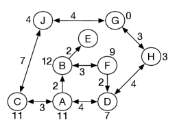
Refer to caption — Figure 3.19: Cyclic delivery graph with node values computed by dynamic programming. Each node $n$ is shown with ${cost\_to\_goal}(n)$

$E$ has no path to $G$ , so there is no value for ${cost\_to\_goal}(E)$ .

A policy is a specification of which arc to take from each node. An optimal policy is a policy such that the cost of following that policy is not worse than the cost of following any other policy. Given a ${cost\_to\_goal}$ function, which is computed offline, a policy can be computed as follows: From node $n$ it should go to a neighbor $m$ that minimizes ${cost}(\left<n,m\right>)+{cost\_to\_goal}(m)$ . This policy will take the agent from any node to a goal along a lowest-cost path.

Either this neighbor can be recorded for all nodes offline, and the mapping from node to node is provided to the agent for online action, or the ${cost\_to\_goal}$ function is given to the agent and each neighbor can be computed online.

Dynamic programming takes time and space linear in the size of the graph to build the ${cost\_to\_goal}$ table. Once the ${cost\_to\_goal}$ function has been built, even if the policy has not been recorded, the time to determine which arc is optimal depends only on the number of neighbors for the node.

Example 3.22.

Given the ${cost\_to\_goal}$ of Figure 3.19 for the goal of getting to $G$ , if the agent is at $A$ , it compares $2+12=14$ (the cost of going via $B$ ), $11+3=14$ (the cost of going via $C$ ), and $4+7=11$ (the cost of going straight to $D$ ). So it is shortest to go next to $D$ .

Partial Dynamic Programming as a Source of Heuristics

Dynamic programming does not have to be run to completion to be useful. Suppose ${cost\_to\_goal}(n)$ has a value for every node $n$ that has a path to a goal with cost less than $c$ . Any node that does not have a ${cost\_to\_goal}$ must have a cost of at least $c$ . Suppose $h$ is an admissible heuristic function that satisfies the monotone restriction. Then the heuristic function

h^{\prime}(n)=\left\{\begin{array}[]{ll}{cost\_to\_goal}(n)&\mbox{if }{cost\_% to\_goal}(n)\mbox{ is defined}\\ \max(c,h(n))&\mbox{otherwise}\end{array}\right.

is an admissible heuristic function that satisfies the monotone restriction and, unless $h$ is already perfect for nodes within cost $c$ of a goal, improves $h$ . It is perfect for all values less than $c$ , but uses $h$ for values greater than $c$ . This refined heuristic function can be dramatically more efficient than $h$ .

Another way to build a heuristic function is to simplify the problem by leaving out some details. Dynamic programming can be used to find the cost of an optimal path to a goal in the simplified problem. This information forms a pattern database that can then be used as a heuristic for the original problem.

Dynamic programming is useful when

•

the goal nodes are explicit (the methods based on the generic search algorithm only assumed a function that recognizes goal nodes)
•

a lowest-cost path is needed
•

the graph is finite and small enough to be able to store the ${cost\_to\_goal}$ value for each node
•

the goal does not change very often
•

the policy is used a number of times for each goal, so that the cost of generating the ${cost\_to\_goal}$ values can be amortized over many instances of the problem.

The main problems with dynamic programming are that

•

it only works when the graph is finite and the table can be made small enough to fit into memory
•

an agent must recompute a policy for each different goal
•

the time and space required is linear in the size of the graph, where the graph size for finite graphs can be exponential in the path length.

Artificial Intelligence 3E